Valle-Oganov descriptor

Implementation of the fingerprint descriptor by Valle and Oganov [1] for \(k=2\) and \(k=3\) [2]. Note that the descriptor is implemented as a subclass of MBTR and can also can also be accessed in MBTR by setting the right parameters: see the MBTR tutorial.

It is advisable to first check out the MBTR tutorial to understand the basics of the MBTR framework. The differences compared to MBTR are:

Only geometry functions distance and angle are available.

A radial cutoff distance r_cut is used.

In the grid setup, min is always 0 and max has the same value as r_cut.

Normalization and weighting are automatically set to their Valle-Oganov options.

periodic is set to True: Valle-Oganov normalization doesn’t support non-periodic systems.

Parameters species and sparse work similarly to MBTR.

Setup

Instantiating a Valle-Oganov descriptor can be done as follows:

import numpy as np
from dscribe.descriptors import ValleOganov

# Setup
vo = ValleOganov(
    species=["H", "O"],
    function="distance",
    sigma=10**(-0.5),
    n=100,
    r_cut=5
)

The arguments have the following effect:

ValleOganov.__init__(species, function, n, sigma, r_cut, sparse=False, dtype='float64')[source]

Parameters:

species (iterable) – The chemical species as a list of atomic numbers or as a list of chemical symbols. Notice that this is not the atomic numbers that are present for an individual system, but should contain all the elements that are ever going to be encountered when creating the descriptors for a set of systems. Keeping the number of chemical species as low as possible is preferable.
function (str) –
The geometry function. The order \(k\) tells how many atoms are involved in the calculation and thus also heavily influence the computational time.

The following geometry functions are available:
- \(k=2\)
  - "distance": Pairwise distance in angstroms.
- \(k=3\)
  - "angle": Angle in degrees.
n (int) – Number of discretization points.
sigma (float) – Standard deviation of the gaussian broadening
r_cut (float) – Radial cutoff.
sparse (bool) – Whether the output should be a sparse matrix or a dense numpy array.
dtype (str) –
The data type of the output. Valid options are:
- "float32": Single precision floating point numbers.
- "float64": Double precision floating point numbers.

In some publications, a grid parameter \(\Delta\), which signifies the width of the spacing, is used instead of n. However, here n is used in order to keep consistent with MBTR. The correlation between n and \(\Delta\) is \(n=(max-min)/\Delta+1=(r_{cutoff})/\Delta+1\).

Creation

After the descriptor has been set up, it may be used on atomic structures with the create()-method.

from ase import Atoms
import math
water = Atoms(
    cell=[[5.0, 0.0, 0.0], [0.0, 5.0, 0.0], [0.0, 0.0, 5.0]],
    positions=[
        [0, 0, 0],
        [0.95, 0, 0],
        [
            0.95 * (1 + math.cos(76 / 180 * math.pi)),
            0.95 * math.sin(76 / 180 * math.pi),
            0.0,
        ],
    ],
    symbols=["H", "O", "H"],
)

# Create ValleOganov output for the system
vo_water = vo.create(water)

print(vo_water)
print(vo_water.shape)

The call syntax for the create-function is as follows:

MBTR.create(system, n_jobs=1, only_physical_cores=False, verbose=False)[source]

Return MBTR output for the given systems.

Parameters:

system (ase.Atoms or list of ase.Atoms) – One or many atomic structures.
n_jobs (int) – Number of parallel jobs to instantiate. Parallellizes the calculation across samples. Defaults to serial calculation with n_jobs=1. If a negative number is given, the used cpus will be calculated with, n_cpus + n_jobs, where n_cpus is the amount of CPUs as reported by the OS. With only_physical_cores you can control which types of CPUs are counted in n_cpus.
only_physical_cores (bool) – If a negative n_jobs is given, determines which types of CPUs are used in calculating the number of jobs. If set to False (default), also virtual CPUs are counted. If set to True, only physical CPUs are counted.
verbose (bool) – Controls whether to print the progress of each job into to the console.

Returns:

MBTR for the given systems. The return type depends on the ‘sparse’ attribute.

Return type:

np.ndarray | sparse.COO

The output will in this case be a numpy array with shape [n_positions, n_features]. The number of features may be requested beforehand with the get_number_of_features()-method.

Examples

The following examples demonstrate some use cases for the descriptor. These examples are also available in dscribe/examples/valleoganov.py.

Visualization

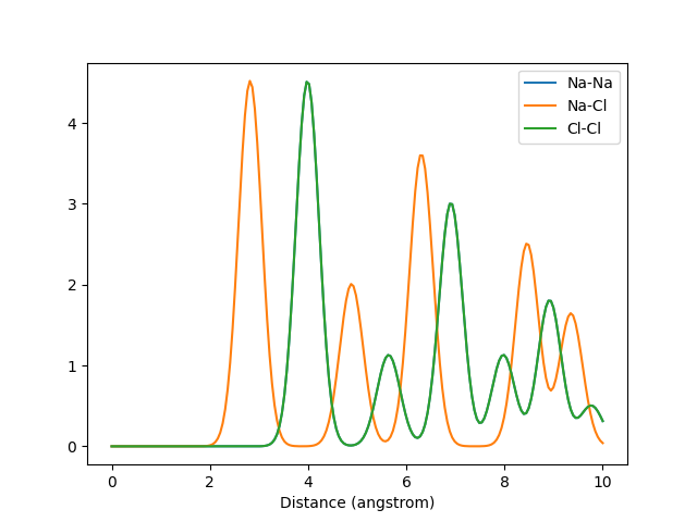
The following snippet demonstrates how the output for \(k=2\) can be visualized with matplotlib. Visualization works very similarly to MBTR.

import matplotlib.pyplot as plt
import ase.data
from ase.build import bulk

nacl = bulk("NaCl", "rocksalt", a=5.64)
vo = ValleOganov(
    species=["Na", "Cl"],
    function="distance",
    n=200,
    sigma=10**(-0.625),
    r_cut=10,
    sparse=False
)
vo_nacl = vo.create(nacl)

# Create the mapping between an index in the output and the corresponding
# chemical symbol
n_elements = len(vo.species)
x = np.linspace(0, 10, 200)

# Plot k=2
fig, ax = plt.subplots()
legend = []
for i in range(n_elements):
    for j in range(n_elements):
        if j >= i:
            i_species = vo.species[i]
            j_species = vo.species[j]
            loc = vo.get_location((i_species, j_species))
            plt.plot(x, vo_nacl[loc])
            legend.append(f'{i_species}-{j_species}')
ax.set_xlabel("Distance (angstrom)")
plt.legend(legend)
plt.show()

Valle-Oganov k=2 — The Valle-Oganov output for k=2. The graphs for Na-Na and Cl-Cl overlap due to their identical arrangement in the crystal.

Setup with MBTR class

For comparison, the setup for Valle-Oganov descriptor for the previous structure, but using the MBTR class, would look like the following.

from dscribe.descriptors import MBTR
mbtr = MBTR(
    species=["Na", "Cl"],
    geometry={"function": "distance"},
    grid={"min": 0, "max": 10, "sigma": 10**(-0.625), "n": 200},
    weighting={"function": "inverse_square", "r_cut": 10},
    normalize_gaussians=True,
    normalization="valle_oganov",
    periodic=True,
    sparse=False
)

mbtr_nacl = mbtr.create(nacl)

Side by side with MBTR output

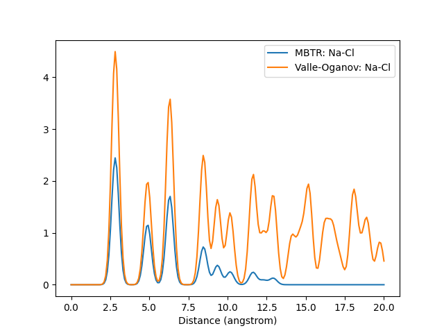
A graph of the output for the same structure created with different descriptors. Also demonstrates how the Valle-Oganov normalization for k2 term converges at 1.

nacl = bulk("NaCl", "rocksalt", a=5.64)

decay = 0.5
mbtr = MBTR(
    species=["Na", "Cl"],
    geometry={"function": "distance"},
    grid={"min": 0, "max": 20, "sigma": 10**(-0.625), "n": 200},
    weighting={"function": "exp", "scale": decay, "threshold": 1e-3},
    periodic=True,
    sparse=False
)

vo = ValleOganov(
    species=["Na", "Cl"],
    function="distance",
    n=200,
    sigma=10**(-0.625),
    r_cut=20,
    sparse=False
)

mbtr_output = mbtr.create(nacl)
vo_output = vo.create(nacl)

n_elements = len(vo.species)
x = np.linspace(0, 20, 200)

fig, ax = plt.subplots()
legend = []
for key, output in {"MBTR": mbtr_output, "Valle-Oganov": vo_output}.items():
    i_species = vo.species[0]
    j_species = vo.species[1]
    loc = vo.get_location((i_species, j_species))
    plt.plot(x, output[loc])
    legend.append(f'{key}: {i_species}-{j_species}')
ax.set_xlabel("Distance (angstrom)")
plt.legend(legend)
plt.show()

Valle-Oganov and MBTR comparison — Outputs for k=2. For the sake of clarity, the cutoff distance has been lengthened and only the Na-Cl pair has been plotted.

[1]

Mario Valle and Artem R Oganov. Crystal fingerprint space–a novel paradigm for studying crystal-structure sets. Acta Crystallographica Section A: Foundations of Crystallography, 66(5):507–517, 2010.

[2]

Malthe K Bisbo and Bjørk Hammer. Global optimization of atomistic structure enhanced by machine learning. arXiv preprint arXiv:2012.15222, 2020.