Supervised Learning: Training an ML Force-field
This tutorial covers how descriptors can be effectively used as input for a machine learning model that will predict energies and forces. There are several design choices that you have to make when building a ML force-field: which ML model, which descriptor, etc. In this tutorial we will use the following, very simple setup:
Dataset of two atoms interacting through a Lennard-Jones potential. This is pretty much as simple as it gets. Real systems will be much more complicated thus requiring a more complicated machine learning model and longer training times.
SOAP descriptor calculated directly between the two atoms. Once again this is for simplicity and in real systems you would have many more centers, possibly on top of each atom.
We will use a fully connected neural network to perform the prediction. In principle any machine learning method will do, but neural networks can very conveniently calculate the analytical derivatives of the output with respect to the input. This allows us to train an energy prediction model from which we will automatically get the forces as long as we also know the derivatives of the descriptor with respect to the atomic positions. This is exactly what the
derivatives-function provided by DScribe returns (notice that DScribe does not yet provide these derivatives for all descriptors).
Setup
We will use a dataset of feature vectors \(\mathbf{D}\), their derivatives \(\nabla_{\mathbf{r_i}} \mathbf{D}\) and the associated system energies \(E\) and forces \(\mathbf{F}\) for training. We will use a neural network \(f\) to predict the energies: \(\hat{E} = f(\mathbf{D})\). Here variables with a “hat” on top indicate predicted quantities to distinguish them from the real values. The predicted forces can be directly computed as the negative gradients with respect to the atomic positions. For example the force for atom \(i\) can be computed as (using row vectors):
In these equations \(\nabla_{\mathbf{D}} f\) is the derivative of the ML model output with respect to the input descriptor. As mentioned before, neural networks typically can output these derivatives analytically. \(\nabla_{\mathbf{r_i}} \mathbf{D}\) is the descriptor derivative with respect to an atomic position. DScribe provides these derivatives for the SOAP descriptor. Notice that in the derivatives provided by DScribe last dimension loops over the features. This makes calculating the involved dot products faster in an environment that uses a row-major order, such as numpy or C/C++, as the dot product is taken over the last, fastest dimension. But you can of course organize the output in any way you like.
The loss function for the neural network will contain the sum of mean squared error of both energies and forces. In order to better equalize the contribution of these two properties in the loss function their values are scaled by their variance in the training set.
Dataset generation
The following script generates our training dataset (full script in the GitHub repository: examples/forces_and_energies/dataset.py):
import numpy as np
import ase
from ase.calculators.lj import LennardJones
import matplotlib.pyplot as plt
from dscribe.descriptors import SOAP
# Setting up the SOAP descriptor
soap = SOAP(
species=["H"],
periodic=False,
r_cut=5.0,
sigma=0.5,
n_max=3,
l_max=0,
)
# Generate dataset of Lennard-Jones energies and forces
n_samples = 200
traj = []
n_atoms = 2
energies = np.zeros(n_samples)
forces = np.zeros((n_samples, n_atoms, 3))
r = np.linspace(2.5, 5.0, n_samples)
for i, d in enumerate(r):
a = ase.Atoms('HH', positions = [[-0.5 * d, 0, 0], [0.5 * d, 0, 0]])
a.set_calculator(LennardJones(epsilon=1.0 , sigma=2.9))
traj.append(a)
energies[i] = a.get_total_energy()
forces[i, :, :] = a.get_forces()
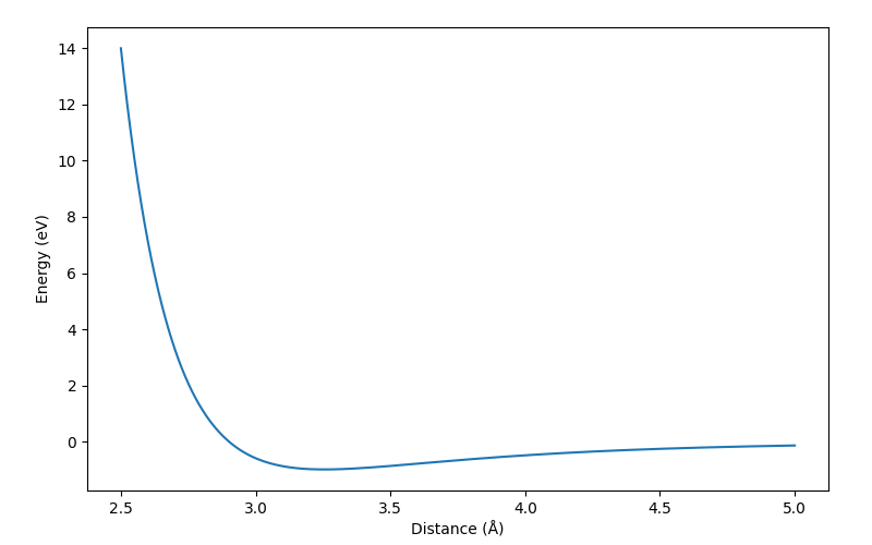
# Plot the energies to validate them
fig, ax = plt.subplots(figsize=(8, 5))
plt.subplots_adjust(left=0.1, right=0.95, top=0.95, bottom=0.1)
line, = ax.plot(r, energies)
plt.xlabel("Distance (Å)")
plt.ylabel("Energy (eV)")
plt.show()
# Create the SOAP desciptors and their derivatives for all samples. One center
# is chosen to be directly between the atoms.
derivatives, descriptors = soap.derivatives(
traj,
centers=[[[0, 0, 0]]] * len(r),
method="analytical"
)
# Save to disk for later training
np.save("r.npy", r)
np.save("E.npy", energies)
np.save("D.npy", descriptors)
np.save("dD_dr.npy", derivatives)
np.save("F.npy", forces)
The energies will look like this:
Training
Note
The training code shown in this tutorial uses pytorch, which you need to install if you wish to run this example. You can find the full script at examples/forces_and_energies/training_pytorch.py. Notice that there is also an identical implementation using tensorflow, kindly provided by xScoschx. It can be found under examples/forces_and_energies/training_tensorflow.py.
Let us first load and prepare the dataset (full script in the GitHub repository: examples/forces_and_energies/training_pytorch.py):
import numpy as np
import torch
from sklearn.preprocessing import StandardScaler
from sklearn.model_selection import train_test_split
torch.manual_seed(7)

# Load the dataset
D_numpy = np.load("D.npy")[:, 0, :]  # We only have one SOAP center
n_samples, n_features = D_numpy.shape
E_numpy = np.array([np.load("E.npy")]).T
F_numpy = np.load("F.npy")
dD_dr_numpy = np.load("dD_dr.npy")[:, 0, :, :, :]  # We only have one SOAP center
r_numpy = np.load("r.npy")

# Select equally spaced points for training
n_train = 30
idx = np.linspace(0, len(r_numpy) - 1, n_train).astype(int)
D_train_full = D_numpy[idx]
E_train_full = E_numpy[idx]
F_train_full = F_numpy[idx]
r_train_full = r_numpy[idx]
dD_dr_train_full = dD_dr_numpy[idx]

# Standardize input for improved learning. Fit is done only on training data,
# scaling is applied to both descriptors and their derivatives on training and
# test sets.
scaler = StandardScaler().fit(D_train_full)
D_train_full = scaler.transform(D_train_full)
D_whole = scaler.transform(D_numpy)
dD_dr_whole = dD_dr_numpy / scaler.scale_[None, None, None, :]
dD_dr_train_full = dD_dr_train_full / scaler.scale_[None, None, None, :]

# Calculate the variance of energy and force values for the training set. These
# are used to balance their contribution to the MSE loss
var_energy_train = E_train_full.var()
var_force_train = F_train_full.var()

# Subselect 20% of validation points for early stopping.
D_train, D_valid, E_train, E_valid, F_train, F_valid, dD_dr_train, dD_dr_valid = train_test_split(
    D_train_full,
    E_train_full,
    F_train_full,
    dD_dr_train_full,
    test_size=0.2,
    random_state=7,
)

# Create tensors for pytorch
D_whole = torch.Tensor(D_whole)
D_train = torch.Tensor(D_train)
D_valid = torch.Tensor(D_valid)
E_train = torch.Tensor(E_train)
E_valid = torch.Tensor(E_valid)
F_train = torch.Tensor(F_train)
F_valid = torch.Tensor(F_valid)
dD_dr_train = torch.Tensor(dD_dr_train)
dD_dr_valid = torch.Tensor(dD_dr_valid)
Then let us define our model and loss function:
class FFNet(torch.nn.Module):
    """A simple feed-forward network with one hidden layer, randomly
    initialized weights, sigmoid activation and a linear output layer.
    """
    def __init__(self, n_features, n_hidden, n_out):
        super(FFNet, self).__init__()
        self.linear1 = torch.nn.Linear(n_features, n_hidden)
        torch.nn.init.normal_(self.linear1.weight, mean=0, std=1.0)
        self.sigmoid = torch.nn.Sigmoid()
        self.linear2 = torch.nn.Linear(n_hidden, n_out)
        torch.nn.init.normal_(self.linear2.weight, mean=0, std=1.0)

    def forward(self, x):
        x = self.linear1(x)
        x = self.sigmoid(x)
        x = self.linear2(x)

        return x


def energy_force_loss(E_pred, E_train, F_pred, F_train):
    """Custom loss function that targets both energies and forces.
    """
    energy_loss = torch.mean((E_pred - E_train)**2) / var_energy_train
    force_loss = torch.mean((F_pred - F_train)**2) / var_force_train
    return energy_loss + force_loss


# Initialize model
model = FFNet(n_features, n_hidden=5, n_out=1)

# The Adam optimizer is used for training the model parameters
optimizer = torch.optim.Adam(model.parameters(), lr=1e-2)
Now we can define the training loop that uses batches and early stopping to prevent overfitting:
# Train!
n_max_epochs = 5000
batch_size = 2
patience = 20
i_worse = 0
old_valid_loss = float("Inf")
best_valid_loss = float("Inf")

# We explicitly require that the gradients should be calculated for the input
# variables. PyTorch will not do this by default as it is typically not needed.
D_valid.requires_grad = True

# Epochs
for i_epoch in range(n_max_epochs):

    # Batches
    permutation = torch.randperm(D_train.size()[0])
    for i in range(0, D_train.size()[0], batch_size):

        indices = permutation[i:i + batch_size]
        D_train_batch, E_train_batch = D_train[indices], E_train[indices]
        D_train_batch.requires_grad = True
        F_train_batch, dD_dr_train_batch = F_train[indices], dD_dr_train[indices]

        # Forward pass: Predict energies from the descriptor input
        E_train_pred_batch = model(D_train_batch)

        # Get derivatives of model output with respect to input variables. The
        # torch.autograd.grad-function can be used for this, as it returns the
        # gradients of the input with respect to outputs. It is very important
        # to set the create_graph=True in this case. Without it the derivatives
        # of the NN parameters with respect to the loss from the force error
        # will not be populated (=the force error will not affect the
        # training), but the model will still run fine without errors.
        df_dD_train_batch = torch.autograd.grad(
            outputs=E_train_pred_batch,
            inputs=D_train_batch,
            grad_outputs=torch.ones_like(E_train_pred_batch),
            create_graph=True,
        )[0]

        # Get derivatives of input variables (=descriptor) with respect to atom
        # positions = forces
        F_train_pred_batch = -torch.einsum('ijkl,il->ijk', dD_dr_train_batch, df_dD_train_batch)

        # Zero gradients, perform a backward pass, and update the weights.
        # D_train_batch.grad.data.zero_()
        optimizer.zero_grad()
        loss = energy_force_loss(E_train_pred_batch, E_train_batch, F_train_pred_batch, F_train_batch)
        loss.backward()
        optimizer.step()

    # Check early stopping criterion and save best model
    E_valid_pred = model(D_valid)
    df_dD_valid = torch.autograd.grad(
        outputs=E_valid_pred,
        inputs=D_valid,
        grad_outputs=torch.ones_like(E_valid_pred),
    )[0]
    F_valid_pred = -torch.einsum('ijkl,il->ijk', dD_dr_valid, df_dD_valid)
    valid_loss = energy_force_loss(E_valid_pred, E_valid, F_valid_pred, F_valid)
    if valid_loss < best_valid_loss:
        # print("Saving at epoch {}".format(i_epoch))
        torch.save(model.state_dict(), "best_model.pt")
        best_valid_loss = valid_loss
    if valid_loss >= old_valid_loss:
        i_worse += 1
    else:
        i_worse = 0
    if i_worse > patience:
        print("Early stopping at epoch {}".format(i_epoch))
        break
    old_valid_loss = valid_loss

    if i_epoch % 500 == 0:
        print("  Finished epoch: {} with loss: {}".format(i_epoch, loss.item()))
Once the model is trained (takes around thirty seconds), we can load the best model and produce predicted data that is saved on disk for later analysis:
# Way to tell pytorch that we are entering the evaluation phase
model.load_state_dict(torch.load("best_model.pt"))
model.eval()

# Calculate energies and force for the entire range
E_whole = torch.Tensor(E_numpy)
F_whole = torch.Tensor(F_numpy)
dD_dr_whole = torch.Tensor(dD_dr_whole)
D_whole.requires_grad = True
E_whole_pred = model(D_whole)
df_dD_whole = torch.autograd.grad(
    outputs=E_whole_pred,
    inputs=D_whole,
    grad_outputs=torch.ones_like(E_whole_pred),
)[0]
F_whole_pred = -torch.einsum('ijkl,il->ijk', dD_dr_whole, df_dD_whole)
E_whole_pred = E_whole_pred.detach().numpy()
E_whole = E_whole.detach().numpy()

# Save results for later analysis
np.save("r_train_full.npy", r_train_full)
np.save("E_train_full.npy", E_train_full)
np.save("F_train_full.npy", F_train_full)
np.save("E_whole_pred.npy", E_whole_pred)
np.save("F_whole_pred.npy", F_whole_pred)
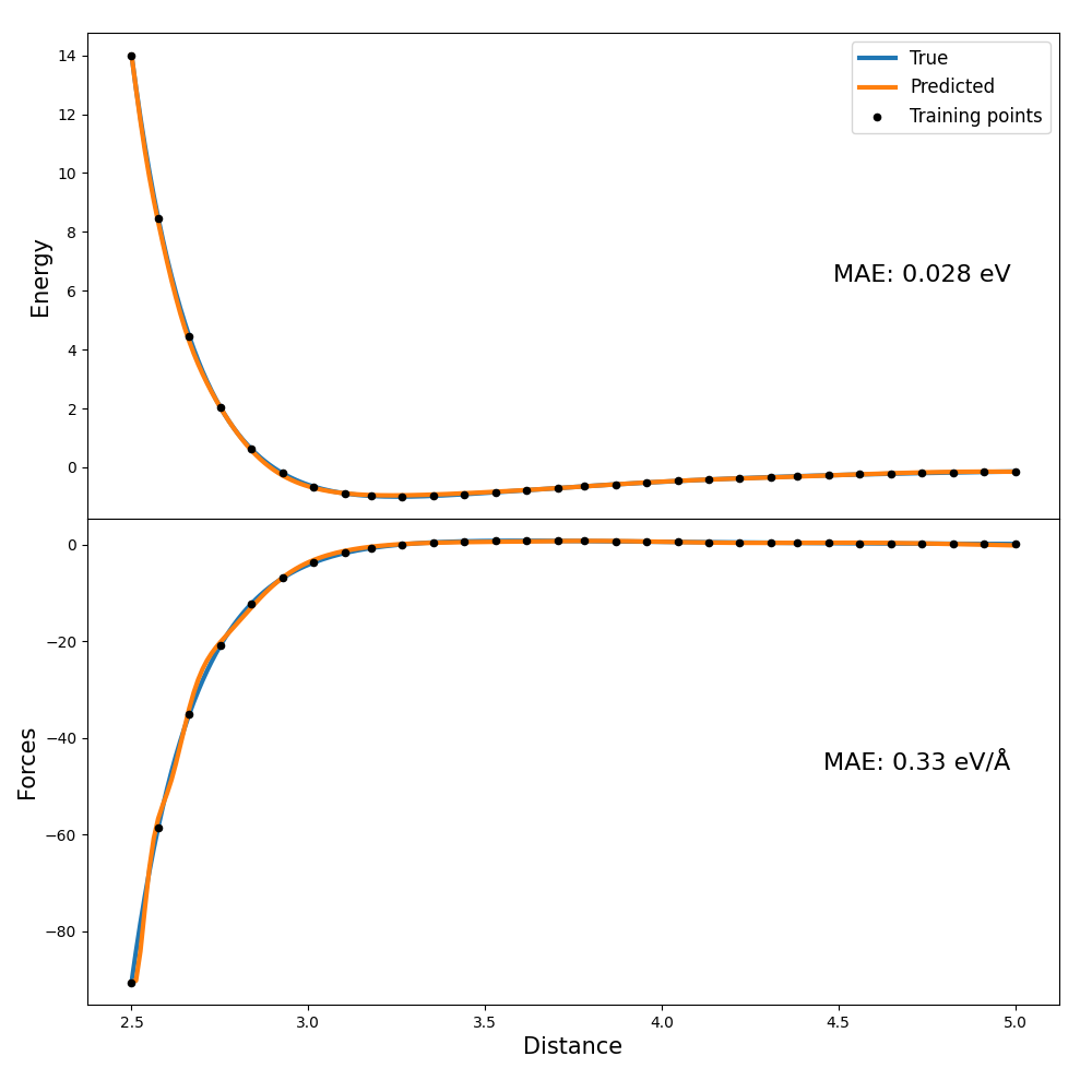
Analysis
In order to quickly assess the model performance, we will simply plot the model response in the whole dataset input domain and compare it to the correct values (full script in the GitHub repository: examples/forces_and_energies/analysis.py):
import numpy as np
from matplotlib import pyplot as plt
from sklearn.metrics import mean_absolute_error

# Load data as produded by the trained model
r_whole = np.load("r.npy")
r_train_full = np.load("r_train_full.npy")
order = np.argsort(r_whole)
E_whole = np.load("E.npy")
E_train_full = np.load("E_train_full.npy")
E_whole_pred = np.load("E_whole_pred.npy")
F_whole = np.load("F.npy")
F_train_full = np.load("F_train_full.npy")
F_whole_pred = np.load("F_whole_pred.npy")
F_x_whole_pred = F_whole_pred[order, 0, 0]
F_x_whole = F_whole[:, 0, 0][order]
F_x_train_full = F_train_full[:, 0, 0]

# Plot energies for the whole range
order = np.argsort(r_whole)
fig, (ax1, ax2) = plt.subplots(2, 1, sharex=True, figsize=(10, 10))
ax1.plot(r_whole[order], E_whole[order], label="True", linewidth=3, linestyle="-")
ax1.plot(r_whole[order], E_whole_pred[order], label="Predicted", linewidth=3, linestyle="-")
ax1.set_ylabel('Energy', size=15)
mae_energy = mean_absolute_error(E_whole_pred, E_whole)
ax1.text(0.95, 0.5, "MAE: {:.2} eV".format(mae_energy), size=16, horizontalalignment='right', verticalalignment='center', transform=ax1.transAxes)

# Plot forces for whole range
ax2.plot(r_whole[order], F_x_whole, label="True", linewidth=3, linestyle="-")
ax2.plot(r_whole[order], F_x_whole_pred, label="Predicted", linewidth=3, linestyle="-")
ax2.set_xlabel('Distance', size=15)
ax2.set_ylabel('Forces', size=15)
mae_force = mean_absolute_error(F_x_whole_pred, F_x_whole)
ax2.text(0.95, 0.5, "MAE: {:.2} eV/Å".format(mae_force), size=16, horizontalalignment='right', verticalalignment='center', transform=ax2.transAxes)

# Plot training points
ax1.scatter(r_train_full, E_train_full, marker="o", color="k", s=20, label="Training points", zorder=3)
ax2.scatter(r_train_full, F_x_train_full, marker="o", color="k", s=20, label="Training points", zorder=3)

# Show plot
ax1.legend(fontsize=12)
plt.subplots_adjust(left=0.08, right=0.97, top=0.97, bottom=0.08, hspace=0)
plt.show()
The plots look something like this: