Unsupervised Learning: Clustering
In this tutorial we take a look at how the descriptors can be used to perform a common unsupervised learning task called clustering. In clustering we are using an unlabeled dataset of input values – in this case the feature vectors that DScribe outputs – to train a model that organizes these inputs into meaningful groups/clusters.
Setup
We will try to find structurally similar locations on top of an copper FCC(111)-surface. To do this, we will first calculate a set of SOAP vectors on top of the surface. To simplify things, we will only consider a single plane 1 Å above the topmost atoms. This set of feature vectors will be our dataset.
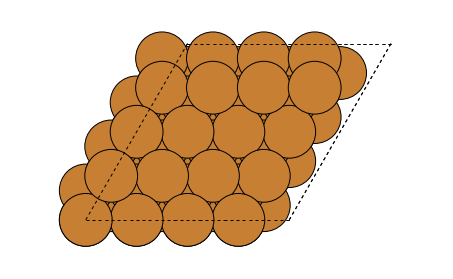
The used copper FCC(111) surface as viewed from above.
This dataset will be used as input for a clustering model. We will use one of the most common and simplest models: k-means clustering. The goal is to use this model to categorize all of the sampled sites into a fixed subset of clusters. We will fix the number of clusters to ten, but this could be changed or even determined dynamically if we used some other clustering algorithm.
As with all forms of unsupervised learning, we do not have the “correct” answers that we could optimize our model againsts. There are certain ways to measure the clustering model performance even without correctly labeled data, but in this simple example we will simply use a setup that provides a reasonable result in our opinion: this is essentially biasing our model.
Dataset generation
The following script generates our training dataset:
import numpy as np
import ase
import ase.build
from ase import Atoms
from ase.visualize import view
from dscribe.descriptors import SOAP


# Lets create an FCC(111) surface
a=3.597
system = ase.build.fcc111(
    "Cu",
    (4,4,4),
    a=3.597,
    vacuum=10,
    periodic=True
)

# Setting up the SOAP descriptor
soap = SOAP(
    sigma=0.1,
    n_max=12,
    l_max=12,
    weighting={"function": "poly", "r0": 12, "m": 2, "c": 1, "d": 1},
    species=["Cu"],
    periodic=True,
)

# Scan the surface in a 2D grid 1 Å above the top-most atom
n = 100
cell = system.get_cell()
top_z_scaled = (system.get_positions()[:, 2].max() + 1) / cell[2, 2]
range_xy = np.linspace(0, 1, n)
x, y, z = np.meshgrid(range_xy, range_xy, [top_z_scaled])
positions_scaled = np.vstack([x.ravel(), y.ravel(), z.ravel()]).T
positions_cart = cell.cartesian_positions(positions_scaled)

# Create the SOAP desciptors for all atoms in the sample.
D = soap.create(system, positions_cart)

# Save to disk for later training
np.save("r.npy", positions_cart)
np.save("D.npy", D)
Training
Let’s load the dataset and fit our model:
import numpy as np
from matplotlib import pyplot as plt
from sklearn.preprocessing import StandardScaler
from sklearn.model_selection import train_test_split
from sklearn.metrics import mean_absolute_error
from sklearn.manifold import TSNE
from sklearn.cluster import MiniBatchKMeans, SpectralClustering, DBSCAN
from matplotlib import cm
from matplotlib.colors import ListedColormap

# Load the dataset
D = np.load("D.npy")
r = np.load("r.npy")
n_samples, n_features = D.shape

# Split into different cluster with K-means
n_clusters = 10
model = MiniBatchKMeans(n_clusters=n_clusters, random_state=42)
model.fit(D)
labels = model.labels_
Analysis
When the training is done (takes few seconds), we can visually examine the clustering. Here we simply plot the sampled points and colour them based on the cluster that was assigned by our model.
# Visualize clusters in a plot
x = r[:, 0]
y = r[:, 1]
colours = cm.get_cmap('viridis', n_clusters)
classes = ["Cluster {}".format(i) for i in range(n_clusters)]
fig, ax = plt.subplots(1,1, figsize=(10, 6))
ax.set_xlabel("x (Å)")
ax.set_ylabel("y (Å)")
ax.axis('equal')
scatter = ax.scatter(x, y, c=labels, cmap=colours, s=15)
ax.legend(handles=scatter.legend_elements()[0], labels=classes)
fig.tight_layout()
plt.show()
The resulting clustering looks like this:
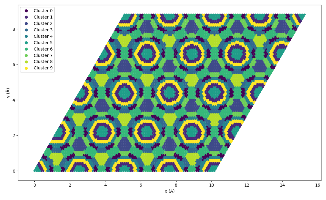
The k-means clustering result.
We can see that our simple clustering setup is able to determine similar regions in our sampling plane. Effectively we have reduced the plane into ten different regions, from which we could select e.g. one representative point per region for further sampling. This provides a powerful tool for pre-selecting informative samples containing chemically and structurally dinstinct sites for e.g. supervised training.