Chemical Environment Visualization with Local Descriptors

This tutorial demonstrates how one can visualize the abstract descriptor feature space by mapping it into a visual property. The goal is to give a rough idea on how to achieve this in a fairly easy scenario where the interesting structural parts are already known and the system does not contain very many different phases of interest. In principle the same technique can however be applied to much more complicated scenarios by using clustering to automatically determine the reference structures and by mapping reference landmarks in the descriptor space into any combination of different visual properties, e.g. fill color, opacity, outline color, size etc.

References and final system

We start out by creating bulk systems for two different iron phases: one for BCC and another for FCC:

import numpy as np
import ase.io
from ase.build import bulk
from dscribe.descriptors import LMBTR

# Lets create iron in BCC phase
n_z = 8
n_xy_bcc = 10
a_bcc = 2.866
bcc = bulk("Fe", "bcc", a=a_bcc, cubic=True) * [n_xy_bcc, n_xy_bcc, n_z]

# Lets create iron in FCC phase
a_fcc = 3.5825
n_xy_fcc = 8
fcc = bulk("Fe", "fcc", a=a_fcc, cubic=True) * [n_xy_fcc, n_xy_fcc, n_z]

Since we know the phases we are looking for a priori, we can simply calculate the reference descriptors for these two environments directly. Here we are using the LMBTR descriptor, but any local descriptor would do:

# Setting up the descriptor
descriptor = LMBTR(
    grid={"min": 0, "max": 12, "sigma": 0.1, "n": 200},
    geometry={"function": "distance"},
    weighting={"function": "exp", "scale": 0.5, "threshold": 1e-3},
    species=["Fe"],
    periodic=True,
)

# Calculate feature references
bcc_features = descriptor.create(bcc, [0])
fcc_features = descriptor.create(fcc, [0])

In the more interesting case where the phases are not known in advance, one could perform some form of clustering (see the tutorial on clustering) to automatically find out meaningful reference structures from the data itself. Next we create a larger system that contains these two grains with a bit of added noise in the atom positions:

# Combine into one large grain boundary system with some added noise
bcc.translate([0, 0, n_z * a_fcc])
combined = bcc + fcc
combined.set_cell([
    n_xy_bcc * a_bcc,
    n_xy_bcc * a_bcc,
    n_z * (a_bcc + a_fcc)
])
combined.rattle(0.1, seed=7)

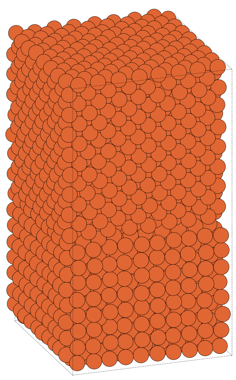
The full structure will look like this:

Coloring

Next we want to generate a simple metric that measures how similar the environment of each atom is to the reference FCC and BCC structures. In this example we define the metric as the Euclidean distance that is scaled to be between 0 and 1 from least similar to identical with reference:

# Create a measure of of how similar the atoms are to the reference. Euclidean
# distance is used and the values are scaled between 0 and 1 from least similar
# to identical with reference.
def metric(values, reference):
    dist = np.linalg.norm(values - reference, axis=1)
    dist_max = np.max(dist)
    return  1 - (dist / dist_max)

Then we calculate the metrics for all atoms in the system:

# Create the features and metrics for all atoms in the sample.
combined_features = descriptor.create(combined)
fcc_metric = metric(combined_features, fcc_features)
bcc_metric = metric(combined_features, bcc_features)

The last step is to create a figure where our custom metric is mapped into colors. We can create an image where the BCC-metric is tied to the blue color, and FCC is tied to red:

# Write an image with the atoms coloured corresponding to their similarity with
# BCC and FCC: BCC = blue, FCC = red
n_atoms = len(combined)
colors = np.zeros((n_atoms, 3))
for i in range(n_atoms):
    colors[i] = [fcc_metric[i], 0, bcc_metric[i]]
ase.io.write(
    f'coloured.png',
    combined,
    rotation='90x,20y,20x',
    colors=colors,
    show_unit_cell=1,
    maxwidth=2000,
)

The final re-colored system looks like this:

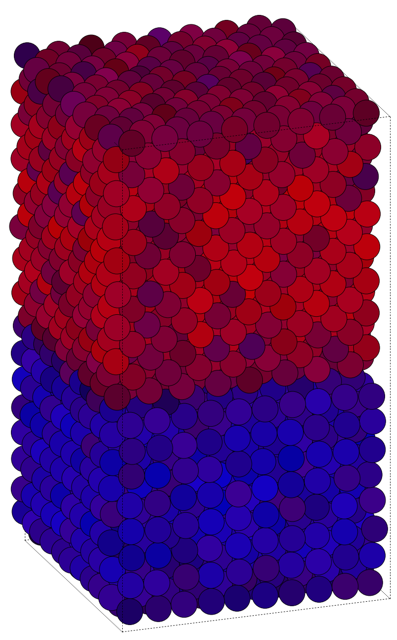
In addition to being able to clearly separate the two grains, one can see imperfections as noise in the coloring and also how the interfaces affect the metric both at the FCC/BCC interface and at the vacuum interface.