Smooth Overlap of Atomic Positions

Smooth Overlap of Atomic Positions (SOAP) is a descriptor that encodes regions of atomic geometries by using a local expansion of a gaussian smeared atomic density with orthonormal functions based on spherical harmonics and radial basis functions.

The SOAP output from DScribe is the partial power spectrum vector \(\mathbf{p}\), where the elements are defined as [1]

\[p^{Z_1 Z_2}_{n n' l} = \pi \sqrt{\frac{8}{2l+1}}\sum_m {c^{Z_1}_{n l m}}^*c^{Z_2}_{n' l m}\]

where \(n\) and \(n'\) are indices for the different radial basis functions up to \(n_\mathrm{max}\), \(l\) is the angular degree of the spherical harmonics up to \(l_\mathrm{max}\) and \(Z_1\) and \(Z_2\) are atomic species.

The coefficients \(c^Z_{nlm}\) are defined as the following inner products:

\[c^Z_{nlm} =\iiint_{\mathcal{R}^3}\mathrm{d}V g_{n}(r)Y_{lm}(\theta, \phi)\rho^Z(\mathbf{r}).\]

where \(\rho^Z(\mathbf{r})\) is the gaussian smoothed atomic density for atoms with atomic number \(Z\) defined as

\[\rho^Z(\mathbf{r}) = \sum_i^{\lvert Z_i \rvert} e^{-1/2\sigma^2 \lvert \mathbf{r} - \mathbf{R}_i \rvert^2}\]

\(Y_{lm}(\theta, \phi)\) are the real spherical harmonics, and \(g_{n}(r)\) is the radial basis function.

For the radial degree of freedom the selection of the basis function \(g_{n}(r)\) is not as trivial and multiple approaches may be used. By default the DScribe implementation uses spherical gaussian type orbitals as radial basis functions [2], as they allow much faster analytic computation. We however also include the possibility of using the original polynomial radial basis set [3].

The spherical harmonics definition used by DScribe is based on real (tesseral) spherical harmonics. This real form spans the same space as the complex version, and is defined as a linear combination of the complex basis. As the atomic density is a real-valued quantity (no imaginary part) it is natural and computationally easier to use this form that does not require complex algebra.

The SOAP kernel [3] between two atomic environments can be retrieved as a normalized polynomial kernel of the partial powers spectrums:

\[K^\mathrm{SOAP}(\mathbf{p}, \mathbf{p'}) = \left( \frac{\mathbf{p} \cdot \mathbf{p'}}{\sqrt{\mathbf{p} \cdot \mathbf{p}~\mathbf{p'} \cdot \mathbf{p'}}}\right)^{\xi}\]

Although this is the original similarity definition, nothing in practice prevents the usage of the output in non-kernel based methods or with other kernel definitions.

Note

Notice that by default the SOAP output by DScribe only contains unique terms, i.e. some terms that would be repeated multiple times due to symmetry are left out. In order to exactly match the original SOAP kernel definition, you have to double the weight of the terms which have a symmetric counter part in \(\mathbf{p}\).

The partial SOAP spectrum ensures stratification of the output by species and also provides information about cross-species interaction. See the get_location() method for a way of easily accessing parts of the output that correspond to a particular species combination. In pseudo-code the ordering of the output vector is as follows:

for Z in atomic numbers in increasing order:
   for Z' in atomic numbers in increasing order:
      for l in range(l_max+1):
         for n in range(n_max):
            for n' in range(n_max):
               if (n', Z') >= (n, Z):
                  append p(\chi)^{Z Z'}_{n n' l}` to output

Setup

Instantiating the object that is used to create SOAP can be done as follows:

from dscribe.descriptors import SOAP

species = ["H", "C", "O", "N"]
r_cut = 6.0
n_max = 8
l_max = 6

# Setting up the SOAP descriptor
soap = SOAP(
    species=species,
    periodic=False,
    r_cut=r_cut,
    n_max=n_max,
    l_max=l_max,
)

The constructor takes the following parameters:

SOAP.__init__(r_cut=None, n_max=None, l_max=None, sigma=1.0, rbf='gto', weighting=None, average='off', compression={'mode': 'off', 'species_weighting': None}, species=None, periodic=False, sparse=False, dtype='float64')

Parameters:

• r_cut (float) – A cutoff for local region in angstroms. Should be bigger than 1 angstrom for the gto-basis.

• n_max (int) – The number of radial basis functions.

• l_max (int) – The maximum degree of spherical harmonics.

• sigma (float) – The standard deviation of the gaussians used to expand the atomic density.

• rbf (str) –

  The radial basis functions to use. The available options are:

  • "gto": Spherical gaussian type orbitals defined as \(g_{nl}(r) = \sum_{n'=1}^{n_\mathrm{max}}\,\beta_{nn'l} r^l e^{-\alpha_{n'l}r^2}\)

  • "polynomial": Polynomial basis defined as \(g_{n}(r) = \sum_{n'=1}^{n_\mathrm{max}}\,\beta_{nn'} (r-r_\mathrm{cut})^{n'+2}\)

• weighting (dict) –

  Contains the options which control the weighting of the atomic density. Leave unspecified if you do not wish to apply any weighting. The dictionary may contain the following entries:

  • "function": The weighting function to use. The following are currently supported:

    • "poly": \(w(r) = \left\{ \begin{array}{ll} c(1 + 2 (\frac{r}{r_0})^{3} -3 (\frac{r}{r_0})^{2}))^{m}, \ \text{for}\ r \leq r_0\\ 0, \ \text{for}\ r > r_0 \end{array}\right.\)

      This function goes exactly to zero at \(r=r_0\). If you do not explicitly provide r_cut in the constructor, r_cut is automatically set to r0. You can provide the parameters c, m and r0 as additional dictionary items.

      For reference see:

      ”Caro, M. (2019). Optimizing many-body atomic descriptors for enhanced computational performance of machine learning based interatomic potentials. Phys. Rev. B, 100, 024112.”

    • "pow": \(w(r) = \frac{c}{d + (\frac{r}{r_0})^{m}}\)

      If you do not explicitly provide r_cut in the constructor, r_cut will be set as the value at which this function decays to the value given by the threshold entry in the weighting dictionary (defaults to 1e-2), You can provide the parameters c, d, m, r0 and threshold as additional dictionary items.

      For reference see:

      ”Willatt, M., Musil, F., & Ceriotti, M. (2018). Feature optimization for atomistic machine learning yields a data-driven construction of the periodic table of the elements. Phys. Chem. Chem. Phys., 20, 29661-29668. “

    • "exp": \(w(r) = \frac{c}{d + e^{-r/r_0}}\)

      If you do not explicitly provide r_cut in the constructor, r_cut will be set as the value at which this function decays to the value given by the threshold entry in the weighting dictionary (defaults to 1e-2), You can provide the parameters c, d, r0 and threshold as additional dictionary items.

  • "w0": Optional weight for atoms that are directly on top of a requested center. Setting this value to zero essentially hides the central atoms from the output. If a weighting function is also specified, this constant will override it for the central atoms.

• average (str) –

  The averaging mode over the centers of interest. Valid options are:

  • "off": No averaging.

  • "inner": Averaging over sites before summing up the magnetic quantum numbers: \(p_{nn'l}^{Z_1,Z_2} \sim \sum_m (\frac{1}{n} \sum_i c_{nlm}^{i, Z_1})^{*} (\frac{1}{n} \sum_i c_{n'lm}^{i, Z_2})\)

  • "outer": Averaging over the power spectrum of different sites: \(p_{nn'l}^{Z_1,Z_2} \sim \frac{1}{n} \sum_i \sum_m (c_{nlm}^{i, Z_1})^{*} (c_{n'lm}^{i, Z_2})\)

• compression (dict) –

  Contains the options which specify the feature compression to apply. Applying compression can slightly reduce the accuracy of models trained on the feature representation but can also dramatically reduce the size of the feature vector and hence the computational cost. Options are:

  • "mode": Specifies the type of compression. This can be one of:

    • "off": No compression; default.

    • "mu2": The SOAP feature vector is generated in an element-agnostic way, so that the size of the feature vector is now independent of the number of elements (see Darby et al. below for details). It is still possible when using this option to construct a feature vector that distinguishes between elements by supplying element-specific weighting under “species_weighting”, see below.

    • "mu1nu1": Implements the mu=1, nu=1 feature compression scheme from Darby et al.: \(p_{inn'l}^{Z_1,Z_2} \sum_m (c_{nlm}^{i, Z_1})^{*} (\sum_z c_{n'lm}^{i, z})\). In other words, each coefficient for each species is multiplied by a “species-mu2” sum over the corresponding set of coefficients for all other species. If this option is selected, features are generated for each center, but the number of features (the size of each feature vector) scales linearly rather than quadratically with the number of elements in the system.

    • "crossover": The power spectrum does not contain cross-species information and is only run over each unique species Z. In this configuration, the size of the feature vector scales linearly with the number of elements in the system.

  • "species_weighting": Either None or a dictionary mapping each species to a species-specific weight. If None, there is no species-specific weighting. If a dictionary, must contain a matching key for each species in the species iterable. The main use of species weighting is to weight each element differently when using the “mu2” option for compression.

  For reference see:

  ”Darby, J.P., Kermode, J.R. & Csányi, G. Compressing local atomic neighbourhood descriptors. npj Comput Mater 8, 166 (2022). https://doi.org/10.1038/s41524-022-00847-y”

• species (iterable) – The chemical species as a list of atomic numbers or as a list of chemical symbols. Notice that this is not the atomic numbers that are present for an individual system, but should contain all the elements that are ever going to be encountered when creating the descriptors for a set of systems. Keeping the number of chemical species as low as possible is preferable.

• periodic (bool) – Set to True if you want the descriptor output to respect the periodicity of the atomic systems (see the pbc-parameter in the constructor of ase.Atoms).

• sparse (bool) – Whether the output should be a sparse matrix or a dense numpy array.

• dtype (str) –

  The data type of the output. Valid options are:

  • "float32": Single precision floating point numbers.

  • "float64": Double precision floating point numbers.

Increasing the arguments n_max and l_max` makes SOAP more accurate but also increases the number of features.

Creation

After SOAP has been set up, it may be used on atomic structures with the create()-method.

from ase.build import molecule

# Molecule created as an ASE.Atoms
water = molecule("H2O")

# Create SOAP output for the system
soap_water = soap.create(water, centers=[0])

print(soap_water)
print(soap_water.shape)

# Create output for multiple system
samples = [molecule("H2O"), molecule("NO2"), molecule("CO2")]
centers = [[0], [1, 2], [1, 2]]
coulomb_matrices = soap.create(samples, centers)            # Serial
coulomb_matrices = soap.create(samples, centers, n_jobs=2)  # Parallel

As SOAP is a local descriptor, it also takes as input a list of atomic indices or positions. If no such positions are defined, SOAP will be created for each atom in the system. The call syntax for the create-method is as follows:

SOAP.create(system, centers=None, n_jobs=1, only_physical_cores=False, verbose=False)

Return the SOAP output for the given systems and given centers.

Parameters:

• system (ase.Atoms or list of ase.Atoms) – One or many atomic structures.

• centers (list) – Centers where to calculate SOAP. Can be provided as cartesian positions or atomic indices. If no centers are defined, the SOAP output will be created for all atoms in the system. When calculating SOAP for multiple systems, provide the centers as a list for each system.

• n_jobs (int) – Number of parallel jobs to instantiate. Parallellizes the calculation across samples. Defaults to serial calculation with n_jobs=1. If a negative number is given, the used cpus will be calculated with, n_cpus + n_jobs, where n_cpus is the amount of CPUs as reported by the OS. With only_physical_cores you can control which types of CPUs are counted in n_cpus.

• only_physical_cores (bool) – If a negative n_jobs is given, determines which types of CPUs are used in calculating the number of jobs. If set to False (default), also virtual CPUs are counted. If set to True, only physical CPUs are counted.

• verbose (bool) – Controls whether to print the progress of each job into to the console.

Returns:

The SOAP output for the given systems and centers. The return type depends on the ‘sparse’-attribute. The first dimension is determined by the amount of centers and systems and the second dimension is determined by the get_number_of_features()-function. When multiple systems are provided the results are ordered by the input order of systems and their positions.

Return type:

np.ndarray | sparse.COO

The output will in this case be a numpy array with shape [n_positions, n_features]. The number of features may be requested beforehand with the get_number_of_features()-method.

Examples

The following examples demonstrate common use cases for the descriptor. These examples are also available in dscribe/examples/soap.py.

Finite systems

Adding SOAP to water is as easy as:

from ase.build import molecule

# Molecule created as an ASE.Atoms
water = molecule("H2O")

# Create SOAP output for the system
soap_water = soap.create(water, centers=[0])

print(soap_water)
print(soap_water.shape)

We are expecting a matrix where each row represents the local environment of one atom of the molecule. The length of the feature vector depends on the number of species defined in species as well as n_max and l_max. You can try by changing n_max and l_max.

# Lets change the SOAP setup and see how the number of features changes
small_soap = SOAP(species=species, r_cut=r_cut, n_max=2, l_max=0)
big_soap = SOAP(species=species, r_cut=r_cut, n_max=9, l_max=9)
n_feat1 = small_soap.get_number_of_features()
n_feat2 = big_soap.get_number_of_features()
print(n_feat1, n_feat2)

Periodic systems

Crystals can also be SOAPed by simply setting periodic=True in the SOAP constructor and ensuring that the ase.Atoms objects have a unit cell and their periodic boundary conditions are set with the pbc-option.

from ase.build import bulk

copper = bulk('Cu', 'fcc', a=3.6, cubic=True)
print(copper.get_pbc())
periodic_soap = SOAP(
    species=[29],
    r_cut=r_cut,
    n_max=n_max,
    l_max=n_max,
    periodic=True,
    sparse=False
)

soap_copper = periodic_soap.create(copper)

print(soap_copper)
print(soap_copper.sum(axis=1))

Since the SOAP feature vectors of each of the four copper atoms in the cubic unit cell match, they turn out to be equivalent.

Weighting

The default SOAP formalism weights the atomic density equally no matter how far it is from the the position of interest. Especially in systems with uniform atomic density this can lead to the atoms in farther away regions dominating the SOAP spectrum. It has been shown [4] that radially scaling the atomic density can help in creating a suitable balance that gives more importance to the closer-by atoms. This idea is very similar to the weighting done in the MBTR descriptor.

The weighting could be done by directly adding a weighting function \(w(r)\) in the integrals:

\[c^Z_{nlm} =\iiint_{\mathcal{R}^3}\mathrm{d}V g_{n}(r)Y_{lm}(\theta, \phi)w(r)\rho^Z(\mathbf{r}).\]

This can, however, complicate the calculation of these integrals considerably. Instead of directly weighting the atomic density, we can weight the contribution of individual atoms by scaling the amplitude of their Gaussian contributions:

\[\rho^Z(\mathbf{r}) = \sum_i^{\lvert Z_i \rvert} w(\lvert \mathbf{R}_i \rvert)e^{-1/2\sigma^2 \lvert \mathbf{r} - \mathbf{R}_i \rvert^2}\]

This approximates the “correct” weighting very well as long as the width of the atomic Gaussians (as determined by sigma) is small compared to the variation in the weighting function \(w(r)\).

DScribe currently supports this latter simplified weighting, with different weighting functions, and a possibility to also separately weight the central atom (sometimes the central atom will not contribute meaningful information and you may wish to even leave it out completely by setting w0=0). Three different weighting functions are currently supported, and some example instances from these functions are plotted below.

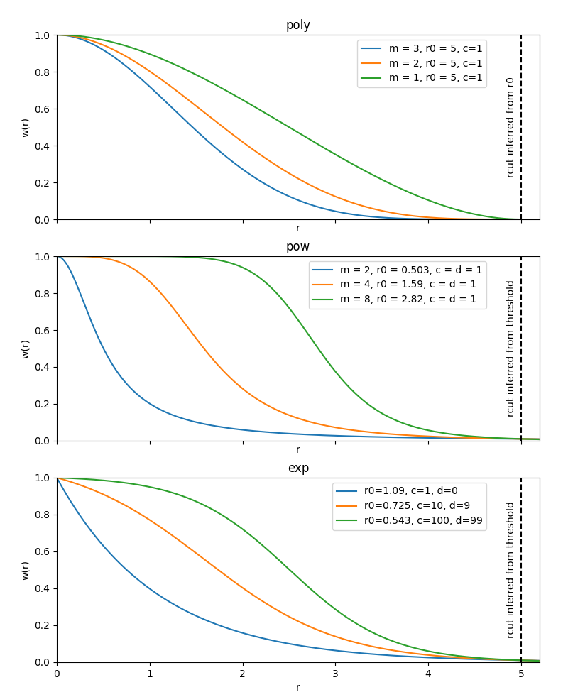
Example instances of weighting functions defined on the interval [0, 1]. The poly function decays exactly to zero at \(r=r_0\), the others decay smoothly towards zero.

When using a weighting function, you typically will also want to restrict r_cut into a range that lies within the domain in which your weighting function is active. You can achieve this by manually tuning r_cut to a range that fits your weighting function, or if you set r_cut=None, it will be set automatically into a sensible range which depends on your weighting function. You can see more details and the algebraic form of the weighting functions in the constructor documentation.

Locating information

The SOAP class provides the get_location()-method. This method can be used to query for the slice that contains a specific element combination. The following example demonstrates its usage.

# The locations of specific element combinations can be retrieved like this.
hh_loc = soap.get_location(("H", "H"))
ho_loc = soap.get_location(("H", "O"))

# These locations can be directly used to slice the corresponding part from an
# SOAP output for e.g. plotting.
soap_water[0, hh_loc]
soap_water[0, ho_loc]

Sparse output

For more information on the reasoning behind sparse output and its usage check our separate documentation on sparse output. Enabling sparse output on SOAP is as easy as setting sparse=True:

soap = SOAP(
    species=species,
    r_cut=r_cut,
    n_max=n_max,
    l_max=l_max,
    sparse=True
)
soap_water = soap.create(water)
print(type(soap_water))

soap = SOAP(
    species=species,
    r_cut=r_cut,
    n_max=n_max,
    l_max=l_max,
    sparse=False
)
soap_water = soap.create(water)
print(type(soap_water))

Average output

One way of turning a local descriptor into a global descriptor is simply by taking the average over all sites. DScribe supports two averaging modes: inner and outer. The inner average is taken over the sites before summing up the magnetic quantum number. Outer averaging instead averages over the power spectrum of individual sites. In general, the inner averaging will preserve the configurational information better but you can experiment with both versions.

average_soap = SOAP(
    species=species,
    r_cut=r_cut,
    n_max=n_max,
    l_max=l_max,
    average="inner",
    sparse=False
)

soap_water = average_soap.create(water)
print("Average SOAP water: ", soap_water.shape)

methanol = molecule('CH3OH')
soap_methanol = average_soap.create(methanol)
print("Average SOAP methanol: ", soap_methanol.shape)

h2o2 = molecule('H2O2')
soap_peroxide = average_soap.create(h2o2)
print("Average SOAP peroxide: ", soap_peroxide.shape)

The result will be a feature vector and not a matrix, so it no longer depends on the system size. This is necessary to compare two or more structures with different number of elements. We can do so by e.g. applying the distance metric of our choice.

from scipy.spatial.distance import pdist, squareform
import numpy as np

molecules = np.vstack([soap_water, soap_methanol, soap_peroxide])
distance = squareform(pdist(molecules))
print("Distance matrix: water - methanol - peroxide: ")
print(distance)

It seems that the local environments of water and hydrogen peroxide are more similar to each other. To see more advanced methods for comparing structures of different sizes with each other, see the kernel building tutorial. Notice that simply averaging the SOAP vector does not always correspond to the Average Kernel discussed in the kernel building tutorial, as for non-linear kernels the order of kernel calculation and averaging matters.

[1]

Sandip De, Albert P. Bartók, Gábor Csányi, and Michele Ceriotti. Comparing molecules and solids across structural and alchemical space. Physical Chemistry Chemical Physics, 18(20):13754–13769, 2016. doi:10.1039/c6cp00415f.

[2]

Marc O J Jäger, Eiaki V Morooka, Filippo Federici Canova, Lauri Himanen, and Adam S Foster. Machine learning hydrogen adsorption on nanoclusters through structural descriptors. npj Computational Materials, 2018. doi:10.1038/s41524-018-0096-5.

[3] (1,2)

Albert P. Bartók, Risi Kondor, and Gábor Csányi. On representing chemical environments. Physical Review B - Condensed Matter and Materials Physics, 87(18):1–16, 2013. doi:10.1103/PhysRevB.87.184115.

[4]

Michael J. Willatt, Félix Musil, and Michele Ceriotti. Feature optimization for atomistic machine learning yields a data-driven construction of the periodic table of the elements. Phys. Chem. Chem. Phys., 20:29661–29668, 2018. doi:10.1039/C8CP05921G.