Sine matrix
The sine matrix [1] captures features of interacting atoms in a periodic system with a very low computational cost. The matrix elements are defined by
Here \(\mathbf{B}\) is a matrix formed by the lattice vectors and \(\hat{\mathbf{e}}_k\) are the cartesian unit vectors. This functional form has no physical interpretation, but it captures some of the properties of the Coulomb interaction, such as the periodicity of the crystal lattice and an infinite energy when two atoms overlap.
Setup
Instantiating the object that is used to create Sine matrices can be done as follows:
from dscribe.descriptors import SineMatrix

# Setting up the sine matrix descriptor
sm = SineMatrix(
    n_atoms_max=6,
    permutation="sorted_l2",
    sparse=False
)
The constructor takes the following parameters:
- SineMatrix.__init__(n_atoms_max, permutation='sorted_l2', sigma=None, seed=None, sparse=False, dtype='float64')
- Parameters:
n_atoms_max (int) – The maximum nuber of atoms that any of the samples can have. This controls how much zeros need to be padded to the final result.
permutation (string) –
Defines the method for handling permutational invariance. Can be one of the following:
none: The matrix is returned in the order defined by the Atoms.
sorted_l2: The rows and columns are sorted by the L2 norm.
eigenspectrum: Only the eigenvalues are returned sorted by their absolute value in descending order.
random: The rows and columns are sorted by their L2 norm after applying Gaussian noise to the norms. The standard deviation of the noise is determined by the sigma-parameter.
sigma (float) – Provide only when using the random-permutation option. Standard deviation of the gaussian distributed noise determining how much the rows and columns of the randomly sorted matrix are scrambled.
seed (int) – Provide only when using the random-permutation option. A seed to use for drawing samples from a normal distribution.
sparse (bool) – Whether the output should be a sparse matrix or a dense numpy array.
Creation
After the Sine matrix has been set up, it may be used on periodic atomic
structures with the create()-method.
from ase.build import bulk

# NaCl crystal created as an ASE.Atoms
nacl = bulk("NaCl", "rocksalt", a=5.64)

# Create output for the system
nacl_sine = sm.create(nacl)

# Create output for multiple system
al = bulk("Al", "fcc", a=4.046)
fe = bulk("Fe", "bcc", a=2.856)
samples = [nacl, al, fe]
sine_matrices = sm.create(samples)            # Serial
sine_matrices = sm.create(samples, n_jobs=2)  # Parallel
The call syntax for the create-function is as follows:
- SineMatrix.create(system, n_jobs=1, only_physical_cores=False, verbose=False)[source]
Return the Sine matrix for the given systems.
- Parameters:
system (
ase.Atomsor list ofase.Atoms) – One or many atomic structures.n_jobs (int) – Number of parallel jobs to instantiate. Parallellizes the calculation across samples. Defaults to serial calculation with n_jobs=1. If a negative number is given, the used cpus will be calculated with, n_cpus + n_jobs, where n_cpus is the amount of CPUs as reported by the OS. With only_physical_cores you can control which types of CPUs are counted in n_cpus.
only_physical_cores (bool) – If a negative n_jobs is given, determines which types of CPUs are used in calculating the number of jobs. If set to False (default), also virtual CPUs are counted. If set to True, only physical CPUs are counted.
verbose (bool) – Controls whether to print the progress of each job into to the console.
- Returns:
Sine matrix for the given systems. The return type depends on the ‘sparse’-attribute. The first dimension is determined by the amount of systems.
- Return type:
np.ndarray | sparse.COO
Note that if you specify in n_atoms_max a lower number than atoms in your
structure it will cause an error. The output will in this case be a flattened
matrix, specifically a numpy array with size n_atoms * n_atoms. The number of
features may be requested beforehand with the
get_number_of_features()-method.
In the case of multiple samples, the creation can also be parallellized by using the
n_jobs-parameter. This splits the list of structures into equally sized parts
and spaws a separate process to handle each part.
Examples
The following examples demonstrate usage of the descriptor. These examples are also available in dscribe/examples/sinematrix.py.
Interaction in a periodic crystal
The following code calculates the interaction value, as defined by the sine matrix, between two aluminum atoms in an FCC-lattice. The values are calculated in the xy-plane.
import numpy as np
from ase import Atoms
import matplotlib.pyplot as mpl
from mpl_toolkits.axes_grid1 import make_axes_locatable

# FCC aluminum crystal
system = bulk("Al", "fcc", cubic=False)

# Calculate the sine matrix entries for a 2D slice at z=0
sm = SineMatrix(
    n_atoms_max=2,
    permutation="none",
    sparse=False
)
n = 100
d = 10
grid = np.zeros((n, n))
values = np.linspace(0, d, n)
for ix, x in enumerate(values):
    for iy, y in enumerate(values):
        i_atom = Atoms(["Al"], positions=[[x, y, 0]])
        i_sys = system.copy()+i_atom
        i_sm = sm.create(i_sys)
        i_sm = sm.unflatten(i_sm)
        i_sm = i_sm[0, 1]
        grid[ix, iy] = i_sm

# Plot the resulting sine matrix values
maxval = 150
fig, ax = mpl.subplots(figsize=(6, 5))
np.clip(grid, a_min=None, a_max=maxval, out=grid)
c1 = ax.contourf(values, values, grid, levels=500)
ax.contour(values, values, grid, levels=5, colors="k", linewidths=0.5, alpha=0.5)
the_divider = make_axes_locatable(ax)
color_axis = the_divider.append_axes("right", size="5%", pad=0.2)
cbar = fig.colorbar(c1, cax=color_axis, ticks=[grid.min(), grid.max()])
ax.axis('equal')
ax.set_ylabel("y (Å)")
ax.set_xlabel("x (Å)")
mpl.tight_layout()
mpl.show()
This code will result in the following plot:
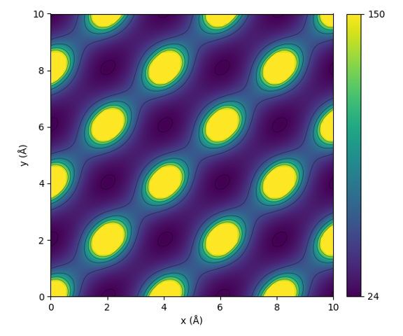
Illustration of the periodic interaction defined by the sine matrix.
From the figure one can see that the sine matrix correctly encodes the periodicity of the lattice. Notice that the shape of the interaction is however not perfectly spherical.
Felix Faber, Alexander Lindmaa, O. Anatole von Lilienfeld, and Rickard Armiento. Crystal structure representations for machine learning models of formation energies. International Journal of Quantum Chemistry, 115(16):1094–1101, 8 2015. doi:10.1002/qua.24917.