Valle-Oganov descriptor

Implementation of the fingerprint descriptor by Valle and Oganov [1] for \(k=2\) and \(k=3\) [2]. Note that the descriptor is implemented as a subclass of MBTR and can also can also be accessed in MBTR by setting the right parameters: see the MBTR tutorial.

It is advisable to first check out the MBTR tutorial to understand the basics of the MBTR framework. The differences compared to MBTR are:

The \(k=1\) term has been removed.

A radial cutoff distance r_cut is used.

In the grid setup, min is always 0 and max has the same value as r_cut.

Normalization and weighting are automatically set to their Valle-Oganov options.

periodic is set to True: Valle-Oganov normalization doesn’t support non-periodic systems.

See below for how to set k2 and k3.

Parameters species, flatten and sparse work similarly to MBTR.

Setup

Instantiating a Valle-Oganov descriptor can be done as follows:

import numpy as np
from dscribe.descriptors import ValleOganov

# Setup
vo = ValleOganov(
    species=["H", "O"],
    k2={
        "sigma": 10**(-0.5),
        "n": 100,
        "r_cut": 5
    },
    k3={
        "sigma": 10**(-0.5),
        "n": 100,
        "r_cut": 5
    },
)

The arguments have the following effect:

In some publications, a grid parameter \(\Delta\), which signifies the width of the spacing, is used instead of n. However, here n is used in order to keep consistent with MBTR. The correlation between n and \(\Delta\) is \(n=(max-min)/\Delta+1=(r_{cutoff})/\Delta+1\).

Creation

After the descriptor has been set up, it may be used on atomic structures with the create()-method.

from ase import Atoms
import math
water = Atoms(
    cell=[[5.0, 0.0, 0.0], [0.0, 5.0, 0.0], [0.0, 0.0, 5.0]],
    positions=[
        [0, 0, 0],
        [0.95, 0, 0],
        [
            0.95 * (1 + math.cos(76 / 180 * math.pi)),
            0.95 * math.sin(76 / 180 * math.pi),
            0.0,
        ],
    ],
    symbols=["H", "O", "H"],
)

# Create ValleOganov output for the system
vo_water = vo.create(water)

print(vo_water)
print(vo_water.shape)

The call syntax for the create-function is as follows:

The output will in this case be a numpy array with shape [#positions, #features]. The number of features may be requested beforehand with the get_number_of_features()-method.

Examples

The following examples demonstrate some use cases for the descriptor. These examples are also available in dscribe/examples/valleoganov.py.

Visualization

The following snippet demonstrates how the output for \(k=2\) can be visualized with matplotlib. Visualization works very similarly to MBTR.

import matplotlib.pyplot as plt
import ase.data
from ase.build import bulk

# The ValleOganov-object is configured with flatten=False so that we can easily
# visualize the different terms.
nacl = bulk("NaCl", "rocksalt", a=5.64)
vo = ValleOganov(
    species=["Na", "Cl"],
    k2={
        "n": 200,
        "sigma": 10**(-0.625),
        "r_cut": 10
    },
    flatten=False,
    sparse=False
)
vo_nacl = vo.create(nacl)

# Create the mapping between an index in the output and the corresponding
# chemical symbol
n_elements = len(vo.species)
imap = vo.index_to_atomic_number
x = np.linspace(0, 10, 200)
smap = {index: ase.data.chemical_symbols[number] for index, number in imap.items()}

# Plot k=2
fig, ax = plt.subplots()
legend = []
for i in range(n_elements):
    for j in range(n_elements):
        if j >= i:
            plt.plot(x, vo_nacl["k2"][i, j, :])
            legend.append(f'{smap[i]}-{smap[j]}')
ax.set_xlabel("Distance (angstrom)")
plt.legend(legend)
plt.show()

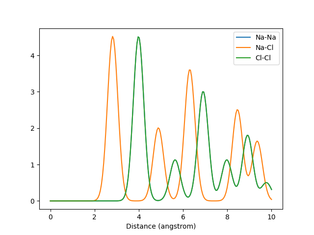
The Valle-Oganov output for k=2. The graphs for Na-Na and Cl-Cl overlap due to their identical arrangement in the crystal.

Setup with MBTR class

For comparison, the setup for Valle-Oganov descriptor for the previous structure, but using the MBTR class, would look like the following.

from dscribe.descriptors import MBTR
mbtr = MBTR(
    species=["Na", "Cl"],
    k2={
        "geometry": {"function": "distance"},
        "grid": {"min": 0, "max": 10, "sigma": 10**(-0.625), "n": 200},
        "weighting": {"function": "inverse_square", "r_cut": 10},
    },
    normalize_gaussians=True,
    normalization="valle_oganov",
    periodic=True,
    flatten=False,
    sparse=False
)

Side by side with MBTR output

A graph of the output for the same structure created with different descriptors. Also demonstrates how the Valle-Oganov normalization for k2 term converges at 1.

nacl = bulk("NaCl", "rocksalt", a=5.64)

decay = 0.5
mbtr = MBTR(
    species=["Na", "Cl"],
    k2={
        "geometry": {"function": "distance"},
        "grid": {"min": 0, "max": 20, "sigma": 10**(-0.625), "n": 200},
        "weighting": {"function": "exp", "scale": decay, "threshold": 1e-3},
    },
    periodic=True,
    flatten=False,
    sparse=False
)

vo = ValleOganov(
    species=["Na", "Cl"],
    k2={
        "n": 200,
        "sigma": 10**(-0.625),
        "r_cut": 20
    },
    flatten=False,
    sparse=False
)

mbtr_output = mbtr.create(nacl)
vo_output = vo.create(nacl)

n_elements = len(vo.species)
imap = vo.index_to_atomic_number
x = np.linspace(0, 20, 200)
smap = {index: ase.data.chemical_symbols[number] for index, number in imap.items()}

fig, ax = plt.subplots()
legend = []
for key, output in {"MBTR": mbtr_output, "Valle-Oganov": vo_output}.items():
    plt.plot(x, output["k2"][0, 1, :])
    legend.append(f'{key}: {smap[0]}-{smap[1]}')
ax.set_xlabel("Distance (angstrom)")
plt.legend(legend)
plt.show()

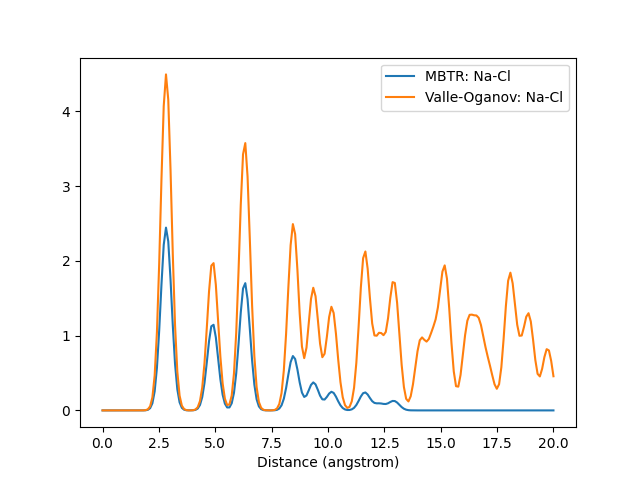
Outputs for k=2. For the sake of clarity, the cutoff distance has been lengthened and only the Na-Cl pair has been plotted.

1: Mario Valle and Artem R Oganov. Crystal fingerprint space–a novel paradigm for studying crystal-structure sets. Acta Crystallographica Section A: Foundations of Crystallography, 66(5):507–517, 2010.
2: Malthe K Bisbo and Bjørk Hammer. Global optimization of atomistic structure enhanced by machine learning. arXiv preprint arXiv:2012.15222, 2020.