Local Many-body Tensor Representation

As the name suggests, the Local Many-body Tensor Representation (LMBTR) is a modification of MBTR for local environments. It is advisable to first check out the MBTR tutorial to understand the basics of the MBTR framework. The main differences compared to MBTR are:

The \(k=1\) term has been removed. Encoding the species present within a local region is quite tricky, and would essentially require some kind of distance information to weight their contribution correctly, making the \(k=1\) term more closer to \(k=2\) term.

LMBTR uses the chemical species X (atomic number 0) for the central position. This makes it possible to also encode spatial locations that are not centered at any particular atom. It does however mean that you should be careful not to mix information from outputs that have different central species. If the chemical identify of the central species is important, you may want to consider a custom output stratification scheme based on the chemical identity of the central species. When used as input for machine learning, training a separate model for each central species is also possible.

Setup

Instantiating an LMBTR descriptor can be done as follows:

import numpy as np
from dscribe.descriptors import LMBTR
from ase.build import bulk
import matplotlib.pyplot as mpl

# Setup
lmbtr = LMBTR(
    species=["H", "O"],
    k2={
        "geometry": {"function": "distance"},
        "grid": {"min": 0, "max": 5, "n": 100, "sigma": 0.1},
        "weighting": {"function": "exp", "scale": 0.5, "threshold": 1e-3},
    },
    k3={
        "geometry": {"function": "angle"},
        "grid": {"min": 0, "max": 180, "n": 100, "sigma": 0.1},
        "weighting": {"function": "exp", "scale": 0.5, "threshold": 1e-3},
    },
    periodic=False,
    normalization="l2_each",
)

The arguments have the following effect:

Creation

After LMBTR has been set up, it may be used on atomic structures with the create()-method.

from ase.build import molecule

water = molecule("H2O")

# Create MBTR output for the system
mbtr_water = lmbtr.create(water, positions=[0])

print(mbtr_water)
print(mbtr_water.shape)

The call syntax for the create-function is as follows:

The output will in this case be a numpy array with shape [#positions, #features]. The number of features may be requested beforehand with the get_number_of_features()-method.

Examples

The following examples demonstrate common use cases for the descriptor. These examples are also available in dscribe/examples/lmbtr.py.

Adsorption site analysis

This example demonstrate the use of LMBTR as a way of analysing local sites in a structure. We build an Al(111) surface and analyze four different adsorption sites on this surface: top, bridge, hcp and fcc.

# Build a surface and extract different adsorption positions
from ase.build import fcc111, add_adsorbate
slab_pure = fcc111('Al', size=(2, 2, 3), vacuum=10.0)
slab_ads = slab_pure.copy()
add_adsorbate(slab_ads, 'H', 1.5, 'ontop')
ontop_pos = slab_ads.get_positions()[-1]
add_adsorbate(slab_ads, 'H', 1.5, 'bridge')
bridge_pos = slab_ads.get_positions()[-1]
add_adsorbate(slab_ads, 'H', 1.5, 'hcp')
hcp_pos = slab_ads.get_positions()[-1]
add_adsorbate(slab_ads, 'H', 1.5, 'fcc')
fcc_pos = slab_ads.get_positions()[-1]

These four sites are described by LMBTR with pairwise \(k=2\) term.

    species=["Al"],
    k2={
        "geometry": {"function": "distance"},
        "grid": {"min": 1, "max": 5, "n": 200, "sigma": 0.05},
        "weighting": {"function": "exp", "scale": 1, "threshold": 1e-2},
    },
    periodic=True,
    normalization="none",
)

# Create output for each site
sites = lmbtr.create(
    slab_pure,
    positions=[ontop_pos, bridge_pos, hcp_pos, fcc_pos],
)

# Plot the site-aluminum distributions for each site

Plotting the output from these sites reveals the different patterns in these sites.

x = lmbtr.get_k2_axis()
mpl.plot(x, sites[0, al_slice], label="top")
mpl.plot(x, sites[1, al_slice], label="bridge")
mpl.plot(x, sites[2, al_slice], label="hcp")
mpl.plot(x, sites[3, al_slice], label="fcc")
mpl.xlabel("Site-Al distance (Å)")
mpl.legend()
mpl.show()

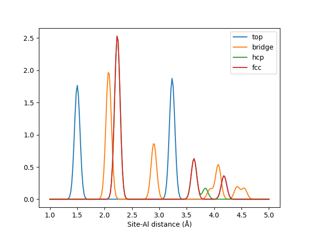
The LMBTR k=2 fingerprints for different adsoprtion sites on an Al(111) surface.

Correctly tuned, such information could for example be used to train an automatic adsorption site classifier with machine learning.