Smooth Overlap of Atomic Positions

Smooth Overlap of Atomic Positions (SOAP) is a descriptor that encodes regions of atomic geometries by using a local expansion of a gaussian smeared atomic density with orthonormal functions based on spherical harmonics and radial basis functions.

The SOAP output from DScribe is the partial power spectrum vector \(\mathbf{p}\), where the elements are defined as [1]

\[p^{Z_1 Z_2}_{n n' l} = \pi \sqrt{\frac{8}{2l+1}}\sum_m {c^{Z_1}_{n l m}}^*c^{Z_2}_{n' l m}\]

where \(n\) and \(n'\) are indices for the different radial basis functions up to \(n_\mathrm{max}\), \(l\) is the angular degree of the spherical harmonics up to \(l_\mathrm{max}\) and \(Z_1\) and \(Z_2\) are atomic species.

The coefficients \(c^Z_{nlm}\) are defined as the following inner products:

\[c^Z_{nlm} =\iiint_{\mathcal{R}^3}\mathrm{d}V g_{n}(r)Y_{lm}(\theta, \phi)\rho^Z(\mathbf{r}).\]

where \(\rho^Z(\mathbf{r})\) is the gaussian smoothed atomic density for atoms with atomic number \(Z\) defined as

\[\rho^Z(\mathbf{r}) = \sum_i^{\lvert Z_i \rvert} e^{-1/2\sigma^2 \lvert \mathbf{r} - \mathbf{R}_i \rvert^2}\]

\(Y_{lm}(\theta, \phi)\) are the real spherical harmonics, and \(g_{n}(r)\) is the radial basis function.

For the radial degree of freedom the selection of the basis function \(g_{n}(r)\) is not as trivial and multiple approaches may be used. By default the DScribe implementation uses spherical gaussian type orbitals as radial basis functions [2], as they allow much faster analytic computation. We however also include the possibility of using the original polynomial radial basis set [3].

The spherical harmonics definition used by DScribe is based on real (tesseral) spherical harmonics. This real form spans the same space as the complex version, and is defined as a linear combination of the complex basis. As the atomic density is a real-valued quantity (no imaginary part) it is natural and computationally easier to use this form that does not require complex algebra.

The SOAP kernel [3] between two atomic environments can be retrieved as a normalized polynomial kernel of the partial powers spectrums:

\[K^\mathrm{SOAP}(\mathbf{p}, \mathbf{p'}) = \left( \frac{\mathbf{p} \cdot \mathbf{p'}}{\sqrt{\mathbf{p} \cdot \mathbf{p}~\mathbf{p'} \cdot \mathbf{p'}}}\right)^{\xi}\]

Although this is the original similarity definition, nothing in practice prevents the usage of the output in non-kernel based methods or with other kernel definitions.

Note

Notice that by default the SOAP output by DScribe only contains unique terms, i.e. some terms that would be repeated multiple times due to symmetry are left out. In order to exactly match the original SOAP kernel definition, you have to double the weight of the terms which have a symmetric counter part in \(\mathbf{p}\).

The partial SOAP spectrum ensures stratification of the output by species and also provides information about cross-species interaction. See the get_location() method for a way of easily accessing parts of the output that correspond to a particular species combination. In pseudo-code the ordering of the output vector is as follows:

for Z in atomic numbers in increasing order:
   for Z' in atomic numbers in increasing order:
      for l in range(l_max+1):
         for n in range(n_max):
            for n' in range(n_max):
               if (n', Z') >= (n, Z):
                  append p(\chi)^{Z Z'}_{n n' l}` to output

Setup

Instantiating the object that is used to create SOAP can be done as follows:

from dscribe.descriptors import SOAP

species = ["H", "C", "O", "N"]
r_cut = 6.0
n_max = 8
l_max = 6

# Setting up the SOAP descriptor
soap = SOAP(
    species=species,
    periodic=False,
    r_cut=r_cut,
    n_max=n_max,
    l_max=l_max,
)

The constructor takes the following parameters:

Increasing the arguments nmax and lmax makes SOAP more accurate but also increases the number of features.

Creation

After SOAP has been set up, it may be used on atomic structures with the create()-method.

from ase.build import molecule

# Molecule created as an ASE.Atoms
water = molecule("H2O")

# Create SOAP output for the system
soap_water = soap.create(water, positions=[0])

print(soap_water)
print(soap_water.shape)

# Create output for multiple system
samples = [molecule("H2O"), molecule("NO2"), molecule("CO2")]
positions = [[0], [1, 2], [1, 2]]
coulomb_matrices = soap.create(samples, positions)            # Serial
coulomb_matrices = soap.create(samples, positions, n_jobs=2)  # Parallel

As SOAP is a local descriptor, it also takes as input a list of atomic indices or positions. If no such positions are defined, SOAP will be created for each atom in the system. The call syntax for the create-method is as follows:

The output will in this case be a numpy array with shape [#positions, #features]. The number of features may be requested beforehand with the get_number_of_features()-method.

Examples

The following examples demonstrate common use cases for the descriptor. These examples are also available in dscribe/examples/soap.py.

Finite systems

Adding SOAP to water is as easy as:

from ase.build import molecule

# Molecule created as an ASE.Atoms
water = molecule("H2O")

# Create SOAP output for the system
soap_water = soap.create(water, positions=[0])

print(soap_water)
print(soap_water.shape)

We are expecting a matrix where each row represents the local environment of one atom of the molecule. The length of the feature vector depends on the number of species defined in species as well as nmax and lmax. You can try by changing nmax and lmax.

# Lets change the SOAP setup and see how the number of features changes
small_soap = SOAP(species=species, r_cut=r_cut, n_max=2, l_max=0)
big_soap = SOAP(species=species, r_cut=r_cut, n_max=9, l_max=9)
n_feat1 = small_soap.get_number_of_features()
n_feat2 = big_soap.get_number_of_features()
print(n_feat1, n_feat2)

Periodic systems

Crystals can also be SOAPed by simply setting periodic=True in the SOAP constructor and ensuring that the ase.Atoms objects have a unit cell and their periodic boundary conditions are set with the pbc-option.

from ase.build import bulk

copper = bulk('Cu', 'fcc', a=3.6, cubic=True)
print(copper.get_pbc())
periodic_soap = SOAP(
    species=[29],
    r_cut=r_cut,
    n_max=n_max,
    l_max=n_max,
    periodic=True,
    sparse=False
)

soap_copper = periodic_soap.create(copper)

print(soap_copper)
print(soap_copper.sum(axis=1))

Since the SOAP feature vectors of each of the four copper atoms in the cubic unit cell match, they turn out to be equivalent.

Weighting

The default SOAP formalism weights the atomic density equally no matter how far it is from the the position of interest. Especially in systems with uniform atomic density this can lead to the atoms in farther away regions dominating the SOAP spectrum. It has been shown [4] that radially scaling the atomic density can help in creating a suitable balance that gives more importance to the closer-by atoms. This idea is very similar to the weighting done in the MBTR descriptor.

The weighting could be done by directly adding a weighting function \(w(r)\) in the integrals:

\[c^Z_{nlm} =\iiint_{\mathcal{R}^3}\mathrm{d}V g_{n}(r)Y_{lm}(\theta, \phi)w(r)\rho^Z(\mathbf{r}).\]

This can, however, complicate the calculation of these integrals considerably. Instead of directly weighting the atomic density, we can weight the contribution of individual atoms by scaling the amplitude of their Gaussian contributions:

\[\rho^Z(\mathbf{r}) = \sum_i^{\lvert Z_i \rvert} w(\lvert \mathbf{R}_i \rvert)e^{-1/2\sigma^2 \lvert \mathbf{r} - \mathbf{R}_i \rvert^2}\]

This approximates the “correct” weighting very well as long as the width of the atomic Gaussians (as determined by sigma) is small compared to the variation in the weighting function \(w(r)\).

DScribe currently supports this latter simplified weighting, with different weighting functions, and a possibility to also separately weight the central atom (sometimes the central atom will not contribute meaningful information and you may wish to even leave it out completely by setting w0=0). Three different weighting functions are currently supported, and some example instances from these functions are plotted below.

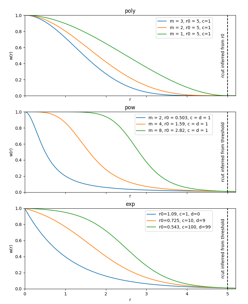
Example instances of weighting functions defined on the interval [0, 1]. The poly function decays exactly to zero at \(r=r_0\), the others decay smoothly towards zero.

When using a weighting function, you typically will also want to restrict r_cut into a range that lies within the domain in which your weighting function is active. You can achieve this by manually tuning r_cut to a range that fits your weighting function, or if you set r_cut=None, it will be set automatically into a sensible range which depends on your weighting function. You can see more details and the algebraic form of the weighting functions in the constructor documentation.

Locating information

The SOAP class provides the get_location()-method. This method can be used to query for the slice that contains a specific element combination. The following example demonstrates its usage.

# The locations of specific element combinations can be retrieved like this.
hh_loc = soap.get_location(("H", "H"))
ho_loc = soap.get_location(("H", "O"))

# These locations can be directly used to slice the corresponding part from an
# SOAP output for e.g. plotting.
soap_water[0, hh_loc]
soap_water[0, ho_loc]

Sparse output

For more information on the reasoning behind sparse output and its usage check our separate documentation on sparse output. Enabling sparse output on SOAP is as easy as setting sparse=True:

soap = SOAP(
    species=species,
    r_cut=r_cut,
    n_max=n_max,
    l_max=l_max,
    sparse=True
)
soap_water = soap.create(water)
print(type(soap_water))

soap = SOAP(
    species=species,
    r_cut=r_cut,
    n_max=n_max,
    l_max=l_max,
    sparse=False
)
soap_water = soap.create(water)
print(type(soap_water))

Average output

One way of turning a local descriptor into a global descriptor is simply by taking the average over all sites. DScribe supports two averaging modes: inner and outer. The inner average is taken over the sites before summing up the magnetic quantum number. Outer averaging instead averages over the power spectrum of individual sites. In general, the inner averaging will preserve the configurational information better but you can experiment with both versions.

average_soap = SOAP(
    species=species,
    r_cut=r_cut,
    n_max=n_max,
    l_max=l_max,
    average="inner",
    sparse=False
)

soap_water = average_soap.create(water)
print("Average SOAP water: ", soap_water.shape)

methanol = molecule('CH3OH')
soap_methanol = average_soap.create(methanol)
print("Average SOAP methanol: ", soap_methanol.shape)

h2o2 = molecule('H2O2')
soap_peroxide = average_soap.create(h2o2)
print("Average SOAP peroxide: ", soap_peroxide.shape)

The result will be a feature vector and not a matrix, so it no longer depends on the system size. This is necessary to compare two or more structures with different number of elements. We can do so by e.g. applying the distance metric of our choice.

from scipy.spatial.distance import pdist, squareform
import numpy as np

molecules = np.vstack([soap_water, soap_methanol, soap_peroxide])
distance = squareform(pdist(molecules))
print("Distance matrix: water - methanol - peroxide: ")
print(distance)

It seems that the local environments of water and hydrogen peroxide are more similar to each other. To see more advanced methods for comparing structures of different sizes with each other, see the kernel building tutorial. Notice that simply averaging the SOAP vector does not always correspond to the Average Kernel discussed in the kernel building tutorial, as for non-linear kernels the order of kernel calculation and averaging matters.

1

Sandip De, Albert P. Bartók, Gábor Csányi, and Michele Ceriotti. Comparing molecules and solids across structural and alchemical space. Physical Chemistry Chemical Physics, 18(20):13754–13769, 2016. doi:10.1039/c6cp00415f.

2

Marc O J Jäger, Eiaki V Morooka, Filippo Federici Canova, Lauri Himanen, and Adam S Foster. Machine learning hydrogen adsorption on nanoclusters through structural descriptors. npj Computational Materials, 2018. doi:10.1038/s41524-018-0096-5.

3(1,2)

Albert P. Bartók, Risi Kondor, and Gábor Csányi. On representing chemical environments. Physical Review B - Condensed Matter and Materials Physics, 87(18):1–16, 2013. doi:10.1103/PhysRevB.87.184115.

4

Michael J. Willatt, Félix Musil, and Michele Ceriotti. Feature optimization for atomistic machine learning yields a data-driven construction of the periodic table of the elements. Phys. Chem. Chem. Phys., 20:29661–29668, 2018. doi:10.1039/C8CP05921G.