Many-body Tensor Representation¶

The many-body tensor representation (MBTR) [1] encodes a structure by using a distribution of different structural motifs. It can be used directly for both finite and periodic systems. MBTR is especially suitable for applications where interpretability of the input is important because the features can be easily visualized and they correspond to specific structural properties of the system.

In MBTR a geometry function \(g_k\) is used to transform a chain of \(k\) atoms, into a single scalar value. The distribution of these scalar values is then constructed with kernel density estimation to represent the structure.

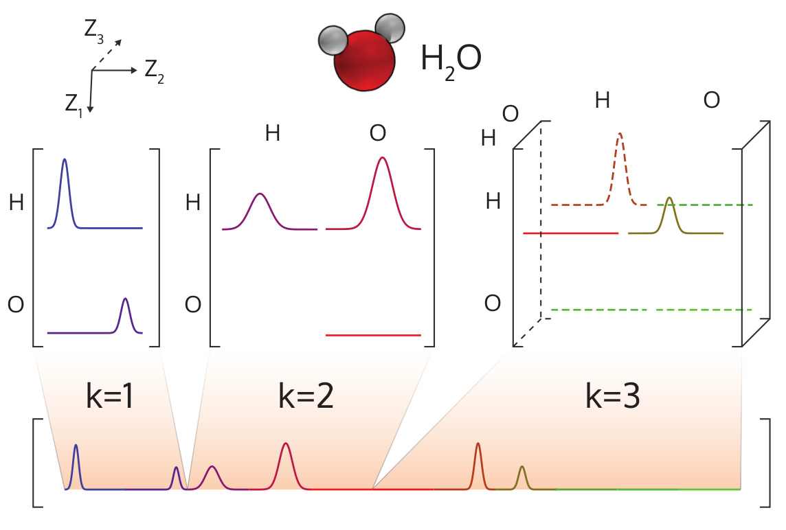
Illustration of the MBTR output for a water molecule.¶

Setup¶

Instantiating an MBTR descriptor can be done as follows:

The arguments have the following effect:

MBTR.__init__(species, periodic, k1=None, k2=None, k3=None, normalize_gaussians=True, normalization='none', flatten=True, sparse=False)[source]¶

Parameters

species (iterable) – The chemical species as a list of atomic numbers or as a list of chemical symbols. Notice that this is not the atomic numbers that are present for an individual system, but should contain all the elements that are ever going to be encountered when creating the descriptors for a set of systems. Keeping the number of chemical speices as low as possible is preferable.
periodic (bool) – Determines whether the system is considered to be periodic.

k1 (dict) –

Setup for the k=1 term. For example:

k1 = {
    "geometry": {"function": "atomic_number"},
    "grid": {"min": 1, "max": 10, "sigma": 0.1, "n": 50}
}

k2 (dict) –

Dictionary containing the setup for the k=2 term. Contains setup for the used geometry function, discretization and weighting function. For example:

k2 = {
    "geometry": {"function": "inverse_distance"},
    "grid": {"min": 0.1, "max": 2, "sigma": 0.1, "n": 50},
    "weighting": {"function": "exp", "scale": 0.75, "cutoff": 1e-2}
}

k3 (dict) –

Dictionary containing the setup for the k=3 term. Contains setup for the used geometry function, discretization and weighting function. For example:

k3 = {
    "geometry": {"function": "angle"},
    "grid": {"min": 0, "max": 180, "sigma": 5, "n": 50},
    "weighting" : {"function": "exp", "scale": 0.5, "cutoff": 1e-3}
}

normalize_gaussians (bool) – Determines whether the gaussians are normalized to an area of 1. Defaults to True. If False, the normalization factor is dropped and the gaussians have the form. \(e^{-(x-\mu)^2/2\sigma^2}\)
normalization (str) –
Determines the method for normalizing the output. The available options are:
- ”none”: No normalization.
- ”l2_each”: Normalize the Euclidean length of each k-term individually to unity.
- ”n_atoms”: Normalize the output by dividing it with the number of atoms in the system. If the system is periodic, the number of atoms is determined from the given unit cell.
flatten (bool) – Whether the output should be flattened to a 1D array. If False, a dictionary of the different tensors is provided, containing the values under keys: “k1”, “k2”, and “k3”:
sparse (bool) – Whether the output should be a sparse matrix or a dense numpy array.

For each k-body term the MBTR class takes in a setup as a dictionary. This dictionary should contain three parts: the geometry function, the grid and the weighting function. The geometry function specifies how the k-body information is encoded. The grid specifies the expected range of the geometry values through the min and max keys. The amount of discretization points is specified with key n and the gaussian smoothing width is specified through the key sigma. The weighting function specifies if and how the different terms should be weighted. Currently the following geometry and weighting functions are available:

The geometry and weighting functions¶
	Geometry functions	Weighting functions
\(k=1\)	“atomic_number”: The atomic numbers.	“unity”: No weighting.
\(k=2\)	“distance”: Pairwise distance in angstroms. “inverse_distance”: Pairwise inverse distance in 1/angstrom.	“unity”: No weighting. “exp” or “exponential”: Weighting of the form \(e^{-sx}\), where x is the distance between the two atoms.
\(k=3\)	“angle”: Angle in degrees. “cosine”: Cosine of the angle.	“unity”: No weighting. “exp” or “exponential”: Weighting of the form \(e^{-sx}\), where x is the perimeter of the triangle formed by the tree atoms.

Creation¶

After MBTR has been set up, it may be used on atomic structures with the create()-method.

The call syntax for the create-function is as follows:

MBTR.create(system, n_jobs=1, verbose=False)[source]¶

Return MBTR output for the given systems.

Parameters

system (ase.Atoms or list of ase.Atoms) – One or many atomic structures.
n_jobs (int) – Number of parallel jobs to instantiate. Parallellizes the calculation across samples. Defaults to serial calculation with n_jobs=1.
verbose (bool) – Controls whether to print the progress of each job into to the console.

Returns

MBTR for the given systems. The return type depends on the ‘sparse’ and ‘flatten’-attributes. For flattened output a single numpy array or sparse scipy.csr_matrix is returned. The first dimension is determined by the amount of systems. If the output is not flattened, dictionaries containing the MBTR tensors for each k-term are returned.

Return type

np.ndarray | scipy.sparse.csr_matrix | list

The output will in this case be a numpy array with shape [#positions, #features]. The number of features may be requested beforehand with the get_number_of_features()-method.

Examples¶

The following examples demonstrate common use cases for the descriptor. These examples are also available in dscribe/examples/mbtr.py.

Locating information¶

If the MBTR setup has been specified with flatten=True, the output is flattened into a single vector and it can become difficult to identify which parts correspond to which element combinations. To overcome this, the MBTR class provides the get_location()-method. This method can be used to query for the slice that contains a specific element combination. The following example demonstrates its usage.

Visualization¶

The MBTR output vector can be visualized easily. The following snippet demonstrates how the output for \(k=2\) can be visualized with matplotlib.

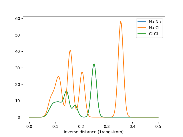
The MBTR output for k=2. The graphs for Na-Na and Cl-Cl overlap due to their identical arrangement in the crystal.¶

Finite systems¶

For finite systems we have to specify periodic=False in the constructor. The need to apply weighting depends on the size of the system: for small systems, such as small molecules, the benefits are small. However for larger systems, such as clusters and bigger molecules, adding weighting will help in removing “noise” coming from atom combinations that are physically very far apart and do not have any meaningful direct interaction in the system. The following code demonstrates both approaches.

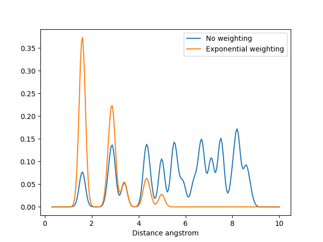
The MBTR output for C60 without weighting and with exponential weighting for \(k=2\). Without the weighting the carbon pairs that are far away will have the highest intensity and dominate the output.¶

Normalization¶

Depending on the application, the preprocessing of the MBTR vector before feeding it into a machine learing model may be beneficial. Normalization is one of the methods that can be used to preprocess the output. Here we go through some examples of what kind of normalization can be used together with MBTR, but ultimately the need for preprocessing depends on both the predicted property and the machine learning algorithm.

The different normalization options provided in the MBTR constructor are:

“none”: No normalization is applied. If the predicted quantity is extensive - scales with the system size - and there is no need to weight the importance of the different \(k\)-terms, then no normalization should be performed.

“l2_each”: Each \(k\)-term is individually scaled to unit Euclidean norm. As the amount of features in the \(k=1\) term scales linearly with number of species, \(k=2\) quadratically and \(k=3\) cubically, the norm can get dominated by the highest \(k\)-term. To equalize the importance of different terms, each \(k\)-term can be individually scaled to unit Euclidean norm. This option can be used if the predicted quantity is intensive - does not scale with the system size, and if the learning method uses the Euclidean norm to determine the similarity of inputs.

“n_atoms”: The whole output is divided by the number of atoms in the system. If the system is periodic, the number of atoms is determined from the given system cell. This form of normalization does also make the output for different crystal supercells equal, but does not equalize the norm of different k-terms.

Periodic systems¶

When applying MBTR to periodic systems, use periodic=True in the constructor. For periodic systems a weighting function needs to be defined, and an exception is raised if it is not given. The weighting essentially determines how many periodic copies of the cell we need to include in the calculation, and without it we would not know when to stop the periodic repetition. The following code demonstrates how to apply MBTR on a periodic crystal:

A problem with periodic crystals that is not directly solved by the MBTR formalism is the fact that multiple different cells shapes and sizes can be used for the same crystal. This means that the descriptor is not unique: the same crystal can have multiple representations in the descriptor space. This can be an issue when predicting properties that do not scale with system size, e.g. band gap or formation energy per atom. The following code and plot demonstrates this for different cells representing the same crystal:

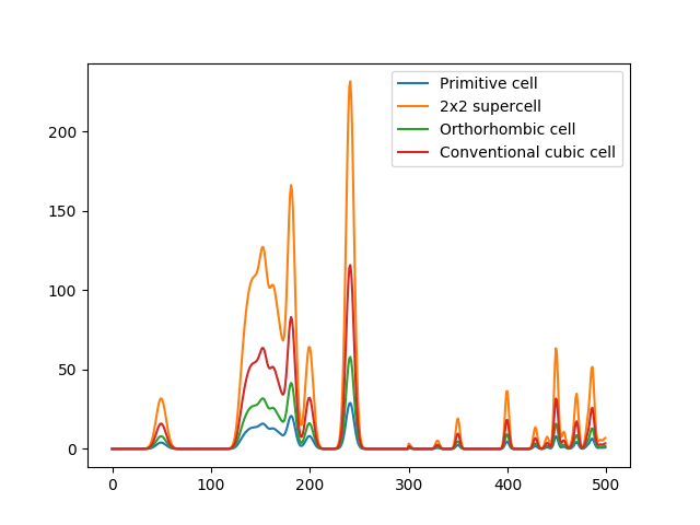
The raw MBTR output for different cells representing the same crystal. The shapes in the output are the same, but the intensities are different (intensities are integer multiples of the primitive system output)¶

However, if the output is normalized (see the example about different normalization methods) we can recover truly identical output for the different cells representing the same material:

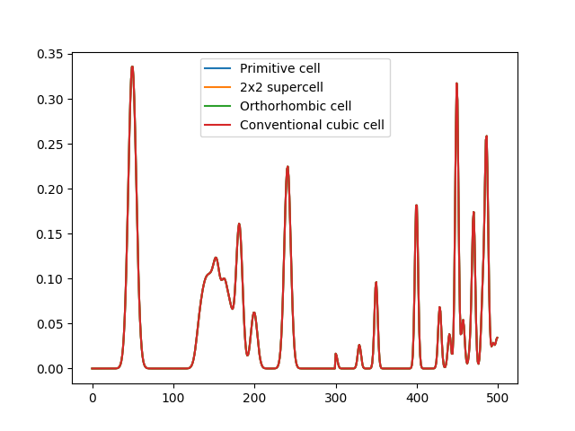
The normalized MBTR output for different cells representing the same crystal. After normalising the output with normalization=’l2_each’, the outputs become identical.¶

DScribe achieves the completely identical MBTR output for different periodic supercells by taking into account the translational multiplicity of the atomic pairs and triples in the system. This is done in practice by weighting the contribution of the pair and triples by how many different periodic repetitions of the original cell are involved in forming the pair or triple.

1: Haoyan Huo and Matthias Rupp. Unified representation of molecules and crystals for machine learning. arXiv e-prints, pages arXiv:1704.06439, Apr 2017. arXiv:1704.06439.