Local Many-body Tensor Representation¶

As the name suggests, the Local Many-body Tensor Representation (LMBTR) is a modification of MBTR for local environments. It is advisable to first check out the MBTR tutorial to understand the basics of the MBTR framework. The main differences compared to MBTR are:

The \(k=1\) term has been removed. Encoding the species present within a local region is quite tricky, and would essentially require some kind of distance information to weight their contribution correctly, making the \(k=1\) term more closer to \(k=2\) term.

LMBTR uses the chemical species X (atomic number 0) for the central position. This makes it possible to also encode spatial locations that are not centered at any particular atom. It does however mean that you should be careful not to mix information from outputs that have different central species. If the chemical identify of the central species is important, you may want to consider a custom output stratification scheme based on the chemical identity of the central species. When used as input for machine learning, training a separate model for each central species is also possible.

Setup¶

Instantiating an LMBTR descriptor can be done as follows:

import numpy as np
from dscribe.descriptors import LMBTR
from ase.build import bulk
import matplotlib.pyplot as mpl

# Setup
lmbtr = LMBTR(
    species=["H", "O"],
    k2={
        "geometry": {"function": "distance"},
        "grid": {"min": 0, "max": 5, "n": 100, "sigma": 0.1},
        "weighting": {"function": "exponential", "scale": 0.5, "cutoff": 1e-3},
    },
    k3={
        "geometry": {"function": "angle"},
        "grid": {"min": 0, "max": 180, "n": 100, "sigma": 0.1},
        "weighting": {"function": "exponential", "scale": 0.5, "cutoff": 1e-3},
    },
    periodic=False,
    normalization="l2_each",
)

The arguments have the following effect:

LMBTR.__init__(species, periodic, k2=None, k3=None, normalize_gaussians=True, normalization='none', flatten=True, sparse=False)[source]¶

Parameters

species (iterable) – The chemical species as a list of atomic numbers or as a list of chemical symbols. Notice that this is not the atomic numbers that are present for an individual system, but should contain all the elements that are ever going to be encountered when creating the descriptors for a set of systems. Keeping the number of chemical speices as low as possible is preferable.
periodic (bool) – Set to true if you want the descriptor output to respect the periodicity of the atomic systems (see the pbc-parameter in the constructor of ase.Atoms).

k2 (dict) –

Dictionary containing the setup for the k=2 term. Contains setup for the used geometry function, discretization and weighting function. For example:

k2 = {
    "geometry": {"function": "inverse_distance"},
    "grid": {"min": 0.1, "max": 2, "sigma": 0.1, "n": 50},
    "weighting": {"function": "exp", "scale": 0.75, "cutoff": 1e-2}
}

k3 (dict) –

Dictionary containing the setup for the k=3 term. Contains setup for the used geometry function, discretization and weighting function. For example:

k3 = {
    "geometry": {"function": "angle"},
    "grid": {"min": 0, "max": 180, "sigma": 5, "n": 50},
    "weighting" = {"function": "exp", "scale": 0.5, "cutoff": 1e-3}
}

normalize_gaussians (bool) – Determines whether the gaussians are normalized to an area of 1. Defaults to True. If False, the normalization factor is dropped and the gaussians have the form. \(e^{-(x-\mu)^2/2\sigma^2}\)
normalization (str) –
Determines the method for normalizing the output. The available options are:
- ”none”: No normalization.
- ”l2_each”: Normalize the Euclidean length of each k-term individually to unity.
flatten (bool) – Whether the output should be flattened to a 1D array. If False, a dictionary of the different tensors is provided, containing the values under keys: “k1”, “k2”, and “k3”:
sparse (bool) – Whether the output should be a sparse matrix or a dense numpy array.

Creation¶

After LMBTR has been set up, it may be used on atomic structures with the create()-method.

from ase.build import molecule

water = molecule("H2O")

# Create MBTR output for the system
mbtr_water = lmbtr.create(water, positions=[0])

print(mbtr_water)
print(mbtr_water.shape)

The call syntax for the create-function is as follows:

LMBTR.create(system, positions=None, n_jobs=1, only_physical_cores=False, verbose=False)[source]¶

Return the LMBTR output for the given systems and given positions.

Parameters

system (ase.Atoms or list of ase.Atoms) – One or many atomic structures.
positions (list) – Positions where to calculate LMBTR. Can be provided as cartesian positions or atomic indices. If no positions are defined, the LMBTR output will be created for all atoms in the system. When calculating LMBTR for multiple systems, provide the positions as a list for each system.
n_jobs (int) – Number of parallel jobs to instantiate. Parallellizes the calculation across samples. Defaults to serial calculation with n_jobs=1. If a negative number is given, the used cpus will be calculated with, n_cpus + n_jobs, where n_cpus is the amount of CPUs as reported by the OS. With only_physical_cores you can control which types of CPUs are counted in n_cpus.
only_physical_cores (bool) – If a negative n_jobs is given, determines which types of CPUs are used in calculating the number of jobs. If set to False (default), also virtual CPUs are counted. If set to True, only physical CPUs are counted.
verbose (bool) – Controls whether to print the progress of each job into to the console.

Returns

The LMBTR output for the given systems and positions. The return type depends on the ‘sparse’-attribute. The first dimension is determined by the amount of positions and systems and the second dimension is determined by the get_number_of_features()-function.

Return type

np.ndarray | scipy.sparse.csr_matrix

The output will in this case be a numpy array with shape [#positions, #features]. The number of features may be requested beforehand with the get_number_of_features()-method.

Examples¶

The following examples demonstrate common use cases for the descriptor. These examples are also available in dscribe/examples/lmbtr.py.

Adsorption site analysis¶

This example demonstrate the use of LMBTR as a way of analysing local sites in a structure. We build an Al(111) surface and analyze four different adsorption sites on this surface: top, bridge, hcp and fcc.

# Build a surface and extract different adsorption positions
from ase.build import fcc111, add_adsorbate
slab_pure = fcc111('Al', size=(2, 2, 3), vacuum=10.0)
slab_ads = slab_pure.copy()
add_adsorbate(slab_ads, 'H', 1.5, 'ontop')
ontop_pos = slab_ads.get_positions()[-1]
add_adsorbate(slab_ads, 'H', 1.5, 'bridge')
bridge_pos = slab_ads.get_positions()[-1]
add_adsorbate(slab_ads, 'H', 1.5, 'hcp')
hcp_pos = slab_ads.get_positions()[-1]
add_adsorbate(slab_ads, 'H', 1.5, 'fcc')
fcc_pos = slab_ads.get_positions()[-1]

These four sites are described by LMBTR with pairwise \(k=2\) term.

    species=["Al"],
    k2={
        "geometry": {"function": "distance"},
        "grid": {"min": 1, "max": 5, "n": 200, "sigma": 0.05},
        "weighting": {"function": "exponential", "scale": 1, "cutoff": 1e-2},
    },
    periodic=True,
    normalization="none",
)

# Create output for each site
sites = lmbtr.create(
    slab_pure,
    positions=[ontop_pos, bridge_pos, hcp_pos, fcc_pos],
)

# Plot the site-aluminum distributions for each site

Plotting the output from these sites reveals the different patterns in these sites.

x = lmbtr.get_k2_axis()
mpl.plot(x, sites[0, al_slice], label="top")
mpl.plot(x, sites[1, al_slice], label="bridge")
mpl.plot(x, sites[2, al_slice], label="hcp")
mpl.plot(x, sites[3, al_slice], label="fcc")
mpl.xlabel("Site-Al distance (Å)")
mpl.legend()
mpl.show()

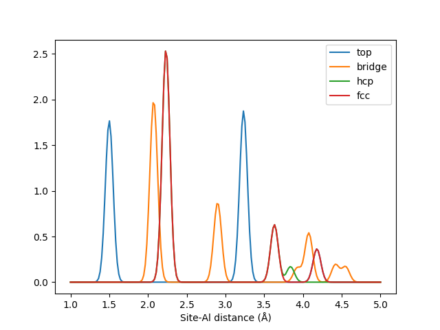
The LMBTR k=2 fingerprints for different adsoprtion sites on an Al(111) surface.¶

Correctly tuned, such information could for example be used to train an automatic adsorption site classifier with machine learning.